This is the official code repository for:
Rose et al. Deep Imputation for Skeleton data (DISK) for behavioral science. Nat Methods (2025). https://doi.org/10.1038/s41592-025-02893-y
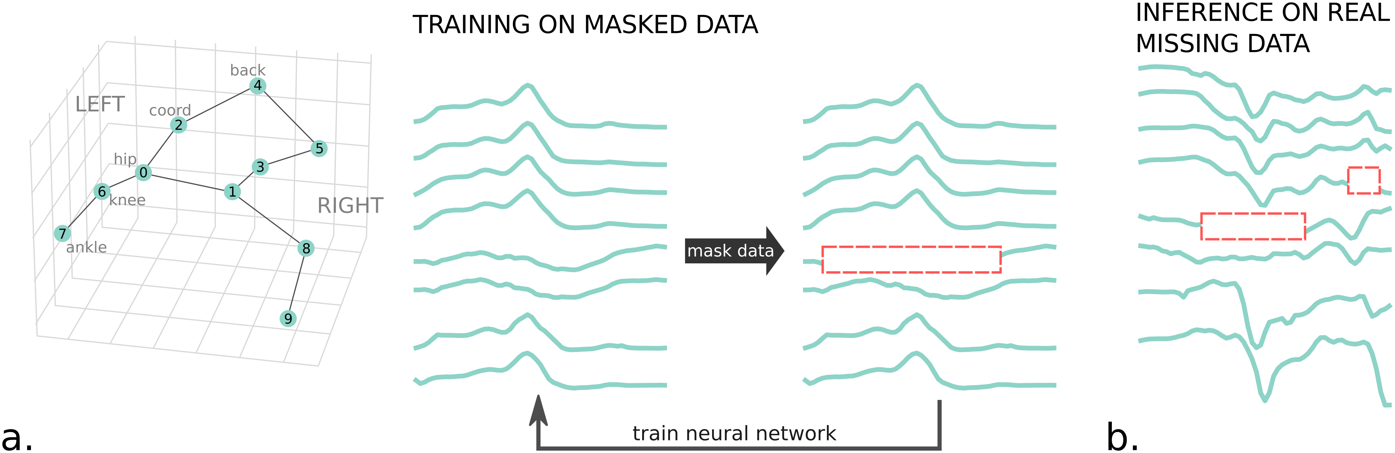
Neural network method to impute missing values for 2D and 3D skeleton data.
 Example of imputations: blue lines are the original signal, red dots represent the imputation done by a transformer model, and the gray line the linear interpolation.
DISK is able to learn correlations between keypoints and dynamics from the training data to fill gaps on a much longer horizon than linear interpolation.
DISK allows to use a bigger proportion of experimental data for downstream behavior analysis.
Example of imputations: blue lines are the original signal, red dots represent the imputation done by a transformer model, and the gray line the linear interpolation.
DISK is able to learn correlations between keypoints and dynamics from the training data to fill gaps on a much longer horizon than linear interpolation.
DISK allows to use a bigger proportion of experimental data for downstream behavior analysis.
pip install disk-imputeTo make DISK work, including PyTorch with the Correct CUDA Backend. First install the correct pytorch for your machine, then pip install disk-impute:
Find link for your CUDA installation at this page Not using a GPU at all?
Installing pytorch can take up to 10-15 minutes.
[VERY IMPORTANT - if using with GPU] To test that pytorch is seeing the GPU, you can test it in a terminal: DISK-check-gpu
If you have trouble installing Pytorch, check this page for pytorch version 1.9.1 and your system.
You can install separately pytorch as a first step using for example
conda install pytorch==1.9.1 cudatoolkit=11.1 -c pytorch -c conda-forge or conda install pytorch==1.9.1 torchvision==0.10.1 torchaudio==0.9.1 cpuonly -c pytorch for the CPU-only version.
For OSX, conda install pytorch==1.9.1 torchvision==0.10.1 torchaudio==0.9.1 -c pytorch or pip install torch==1.9.1 torchvision==0.10.1 torchaudio==0.9.1.
For all cases, test if DISK is installed correctly by running in the terminal:
DISK-check-installThis code allows to train in an unsupervised way a neural network to learn imputation of missing values. Skeleton data are data points corresponding to body parts recorded through time. This code focuses on 3D data.
Several network backbones are implemented:
- Custom Transformer Encoder (transformer) -- best performance,
- Bidirectional Gated Recurrent Unit (GRU) -- 2nd best performance and shorter to train,
- Temporal Convolutional Neural Network (TCN),
- Spatial-Temporal Graph Convolutional Network (ST_GCN),
- Separable Time-Space Graph Convolutional Network (STS_GCN).
These networks have been tested on different animal skeletons and human skeleton (see Datasets section).

The training is done on data with artificially introduced gaps. This process of introducing gaps is controlled by 2 factors:
- the probability of a given keypoint to be missing
- the probability of a given gap length knowing the missing keypoint.
There are 4 main commands:
- DISK-create-project -- creates the folders of the DISK project. Expects a list of input data files.
- DISK-prepare-data -- prepares the data in a DISK-compatible format from the input file list given when created the DISK project.
- DISK-train -- train a DISK model to impute the gaps. Include evaluating and plotting.
- DISK-impute -- impute on original data using the trained model.
Example of command usage (you can run these to see if everything runs without error -- this is not designed to give any good results):
# download the data file to run the demo code
gdown https://drive.google.com/uc?id=1a1iMd_eyVjCXectJjSGKrmP5fpBQkuX_

# create project folder
DISK-create-project --project_path DISK_demo --file_format simple_csv --data_files fish_fighting_interpolated_head_2D.csv

# prepare a dataset for DISK model with a given sample length
DISK-prepare-data --project_path DISK_demo --length 30

# train a DISK model on the previsouly created dataset
DISK-train --project_path DISK_demo --dataset_name dataset_length30_stride15_sequential --training_epochs 3

# use the trained model to impute gaps
DISK-impute --project_path DISK_demo --dataset_name dataset_length30_stride15_sequential --model_name dataset_30_15_DISK
The demo code is to verify that everything works on your machine and to introduce you the main commands.
- The arguments (except training_epochs) are all mandatory. Additionally, there are other parameters to tailor DISK to your situation (see next section.)
- The trained DISK model is not going to perform as it is trained for a very short time on very little data!
There are usual parameters that you might want to set yourself:
At this step, we read the original files, determine the valid portions (without missing data) and crop them in samples of size "length". We also estimate the probability of keypoints missing taken independently or in combination
Additional parameters are:
| parameter name | type, default | description |
|---|---|---|
| dataset_name | string | |
| original_freq | int, in Hz | you can precise the original frequency, will be used for subsampling and plots |
| subsampling_freq | in, in Hz | needs to be lower than original_freq |
| stride | int, between 0 and length | by how many timesteps are separated consecutive samples (after subsampling) |
| fill_gap | int, default: 0 | short gaps under this length will be filled by linear interpolation. This value should be kept small as linear interpolation imprecision grows with length |
| dlc_likelihood_threshold | float, default: 0.9 | if using file_format dlc_csv or dlc_h5, DLC prediction likelihoods falling under this threshold will be considered as missing values |
To compute the probability of missing keypoints, there are two additional parameters:
| parameter name | type, default | description |
|---|---|---|
| indep_keypoints | bool, default: False | if False, look at sets of simultaneous missing keypoints; if True, look at each keypoint independently |
| merge_keypoints | bool, default: False | if True, estimate the probability of n keypoints missing at the same time -- False is preferred unless not enough samples to estimate a good probability |
The syntax remains the same:
DISK-prepare-data --project_path DISK_demo --length 30 --fill_gap 10 --indep_keypoints True
At this step, using a created DISK dataset, a DISK model is trained and evaluated. We advise to run the training on a machine with a GPU.
Additional parameters can be set:
| parameter name | type, default | description |
|---|---|---|
| model_name | str | |
| training_epochs | int, default: 1500 | controls the length of training. The longer the better the results might be. A good practice is to look at the loss curve after a training and see if it has stabilized or if it is still decreasing. In the latter case, additional epochs can be beneficial. You can resume a training using the load_model parameter. |
| load_model | str | name of the model_folder inside the DISK_train folder. To continue the training from a given checkpoint. |
| training_batch_size | int, default: 32 | controls how many samples are loaded in the GPU RAM. Do not touch unless running into out of memory error, then lower this value. |
| n_cpus | int, default: 8 | number of cpus dedicated to DISK. A high number of CPUs will increase the speed of data loading |
| network | str, default: transformer | we advise transformer or gru |
And as in the previous step, you can choose how to compute the probability of missing keypoints with these two additional parameters:
| parameter name | type, default | description |
|---|---|---|
| indep_keypoints | bool, default: False | if False, look at sets of simultaneous missing keypoints; if True, look at each keypoint independently |
| merge_keypoints | bool, default: False | if True, estimate the probability of n keypoints missing at the same time -- False is preferred unless not enough samples to estimate a good probability |
The syntax remains the same:
DISK-train --project_path DISK_demo --dataset_name dataset_30_15 --network gru --n_cpus 1
At this step, we will use a trained DISK model on a given dataset and impute the real gaps.
Additional parameters can be set:
- missing_pad (list of 2 integers, default: [1, 0]) -- how many points to the left and right of the gap is needed for the DISK model to interpolate. Higher numbers will give better precision but fewer imputed gaps. The left value needs to be >= 1.
- n_cpus (int, default: 1) -- used to load the data
- threshold_error_score (float, default: 0.1) -- threshold used to reject bad imputed samples to have an idea about the value to put, look at plots output of the evaluate script (inside
DISK_trainfolder)
- DISK-add-skeleton: prompts the user to enter links between keypoints corresponding to the skeleton. The built skeleton is only used for ST-GCN backbone and plots.
DISK-add-skeleton --project_path ...
- DISK-restore-default-config: restores the original configs inside the config folder
DISK-restore-default-config --project_path ...
- DISK-evaluate: compares different already trained models on a given dataset, outputs plots and metrics
DISK-evaluate --project_path ... --dataset_name ... --model_name_list path/to/model1/folder /path/to/model2/folder
Additionally, a tutorial is available as a Jupyter Notebook and compatible with Google colab: in this github repo in notebooks/DISK_tutorial_2025-05.ipynb
with processed datasets and saved checkpoint models available on zenodo.
Alternatively, the same steps (without the explanations and images) are available as a simple bash script in tests/test_tutorial_zenodo.sh.
This repo uses configuration files (via the hydra package). The log file keeps all the parameters and input values visible at once. These values can be changed by the user and overwritten by the command line as well.
You can set all the values in a config file and use it with the corresponding launcher using this syntax:
DISK-train --config_file path/to/your/yaml/config/file.yaml
All the created files will be saved inside the project directory created with DISK-create-project.
DISK_project_folder
  |
  |_ config_project.yaml
  |
  |_ DISK_data
     |_ dataset_freqF_lengthL_strideS
         |_ train_dataset.npz
         |_ train_fulllength_dataset.npz
         |_ test_dataset.npz
         |_ test_fulllength_dataset.npz
         |_ val_dataset.npz
         |_ val_fulllength_dataset.npz
         |_ constants.py
         |_ dataset_freqF_lengthL_strideS_proba_missing.csv
         |_ dataset_freqF_lengthL_strideS_proba_missing_length.csv
         |
     |_ dataset_1_freqV_lengthW
         |_ ...
         |
     |_ ...
     |
  |_ DISK_train
     |_DISK_model_0
         |_
     |_ DISK_model_1
     |
  |_ DISK_impute
  |
  |_ example_configs
     |_config_impute.yaml
     |_config_prepare_data.yaml
     |_config_train.yaml
-
In the
DISK_datafolder, will be stored each dataset as a folder, e.g.dataset_freqF_lengthL_strideS. In this folderdataset_freqF_lengthL_strideS, the dataset files per se (npz files) and the company files like the one with the dataset constants which will be read when using the dataset (constants.py). -
In the
DISK_datafolder will also be stored the files to create the artificial holes, the files with proba_missing in their names (See Step 2. below).
The accepted formats are:
- .h5 files from SLEAP ('sleap_h5'),
- .h5 and .csv from DeepLabCut (dlc_h5 and dlc_csv),
- .csv files with columns as keypoints coordinates, e.g. 'kp1_x', 'kp1_y', 'kp1_z', 'kp2_x', ...,
- .npy files where only the data are loaded, the keypoints would be named '01', '02', ...,
- .mat files
- other types of formats can be accomodated when a proper opening function is inserted in the function open_and_extract from the script create_dataset.py
This step will prepare the files to input to the neural network. It will prepare the cropped samples without missing data, save the necessary data and metadata in a convenient format.
If ValueError, no data for ... with ... NaNs, probably due to not long enough segments, it means the program has not found segments without any missing data of sufficient length.
Workarounds are:
- decreasing the length,
- do a step of linear imputation before to fill the very small gaps with fill_gaps,
- and/or drop one or several keypoints (the ones with the less good tracking). The length, fill_gaps, and drop_keypoints are options in the config file.
Additionally, if there is enough segments but the resulting datasets have very few training samples (under 1,000) or test/validation samples (under 10). You can further decrease the stride which will create more samples by overlapping them.
On the contrary if the dataset is very large (over 20,000 samples for the training set), then you can increase the stride.
The method has originally been tested on 7 datasets:
- 2 motion capture mouse datasets (FL2 and CLB) with 8 keypoints (in house)
- 1 motion capture rat dataset (Rat7M) with 20 keypoints paper
- 1 motion capture human dataset (MoCap) with 20 keypoints from the CMU Graphics Lab Motion Capture Database downloaded from here
- 1 3D video tracking drosophila dataset (DF3D) with 38 keypoints paper
- 1 3D video tracking 2-Zebrafish dataset(2Fish) with 6 keypoints paper
- 1 3D video tracking 2-mice dataset (2Mice-2D) with 16 keypoints from the AICrowd challenge
Some of them can be directly used to train and test, and are available for download here.
The training will be long, from a few hours to a few days depending on the size of the dataset and the number of required epochs. Hence, we advise to run the training (DISK-train) on a machine with a GPU.
Transformer model has the best performance for all the tested datasets. However, transformer usually benefits from a lower batch size (32 or 64) and is the slowest to train even on GPU. Depending on the size of the training dataset, it can take a few hours to days.
GRU is the second best model in terms of performances. GRU can be trained with larger batch size (up to 512 if enough GPU memory) and is shorter to train. It can still take hours to train on a middle-sized dataset.
To understand loss plots, see FAQ.
DISK-train will automatically output performance metrics of the trained model and plots to investigate the quality of the imputations, on the test subset of the dataset.
The metrics are (log and csv files):
- RMSE (root mean square error) computed per hole. RMSEs per hole will be averaged for the dataset.
- MPJPE (mean per joint position error), this usually correlates with RMSE
- PCK@th (percent of correct keypoints under the threshold th): predicted keypoints at a certain distance from the ground truth will be considered correct. The distance is calculated the fraction th of the maximum distance between two keypoints in a frame for the whole dataset.
The plots represent (png files):
- a barplot to compare averaged RMSE for linear interpolation and the tested model(s)
- a barplot of averaged RMSE per keypoint
- a lineplot of the averaged RMSE with respect to the length of the artificial hole
Randomly selected samples will be plotted showing the ground truth and the imputation(s).

This step should be relatively quick, and can easily be run on CPUs.
Our last step is to impute the real gaps in the original dataset.
Our last step is to impute the real gaps in the original dataset.
Rose, F., Michaluk, M., Blindauer, T. et al. Deep Imputation for Skeleton data (DISK) for behavioral science. Nat Methods (2025). https://doi.org/10.1038/s41592-025-02893-y
Additional scripts to reproduce plots and analyses (comparison with other published methods) are available at: https://github.com/bozeklab/DISK_paper_code
If using conda/pip, you can first create a new environment:
# if using conda environments
conda create --name env_DISK python=3.12 # requires python>=3.8,<3.10
conda activate env_DISK
pip install -e .[dev]
python -m build && unzip dist/disk-<>.whl -d dist/unzipped
twine upload dist/* --config-file .pypirc