class15.jl

### A Pluto.jl notebook ###
# v0.20.20

using Markdown
using InteractiveUtils

macro bind(def, element)
    #! format: off
    return quote
        local iv = try Base.loaded_modules[Base.PkgId(Base.UUID("6e696c72-6542-2067-7265-42206c756150"), "AbstractPlutoDingetjes")].Bonds.initial_value catch; b -> missing; end
        local el = $(esc(element))
        global $(esc(def)) = Core.applicable(Base.get, el) ? Base.get(el) : iv(el)
        el
    end
    #! format: on
end

# ╔═╡ 4866207c-0894-4340-a18b-72f8e1204424
begin
	class_dir = @__DIR__
	import Pkg
	Pkg.activate(".")
	Pkg.instantiate()
	using PlutoUI
	using PlutoTeachingTools
	using MarkdownLiteral
end

# ╔═╡ a1b2c3d4-0894-4340-a18b-72f8e1204425
begin
	using JuMP
	using Ipopt
	using Plots
	using DifferentialEquations
end

# ╔═╡ e6aa5227-91bd-4cec-9448-24384708a305
ChooseDisplayMode()

# ╔═╡ 19dac419-2df3-4878-b7da-608e8ec1e53b
md"""
| | | |
|-----------:|:--|:------------------|
|  Lecturer   | : | Shuaicheng Tong |
|  Topic   | : | Dynamic Optimal Control of Power Systems |
"""

# ╔═╡ 8ed6af99-1c5d-4d27-b60d-17d2e6c6ceff
md"""
## Chapter Outline

This chapter motivates the need for optimization and control of power systems by introducing the **Economic Dispatch (ED)** and **Optimal Power Flow (OPF)** problems and analyzing the physical behaviors they capture in power system.
 
We progressively move from solving *static optimization* problems to augmenting them with *dynamic optimal control* constraints as approaches to analyze and understand power systems.

**Topics covered:**
- **Transients and Transient Stability–Constrained OPF (TSC-OPF):**  
  What are transients, their physical behaviors, and how they are factored into stability analysis of energy systems via the TSC-OPF formulation.

- **Generator Swing Equations:**  
  The physical foundation of synchronous machines — describes how mechanical torque and electrical power control frequency and machine responses to frequency changes.

- **Inverter Control Models:**  
  Grid-following vs. grid-forming inverters, and how virtual inertia control emulates synchronous generator dynamics for renewables.

- **Dynamic Load Models:**  
  Representations of demand that vary with voltage and frequency instead of a fixed a quantity, influencing both stability and control.

> 🧭 **Overall goal:**  
> To connect steady-state optimization (ED/DC-OPF) with **dynamic optimal control**, illustrating how classical control laws and physics-based constraints shape modern power system operation.
"""

# ╔═╡ f742f5f3-d9d3-4374-ac9e-17073c3a2f6d
md"""
# Introduction to Energy Systems
## From Economic Dispatch to Dynamic Optimal Control

Optimal control of power systems builds on static optimization formulations like *economic dispatch* (ED) and *optimal power flow* (OPF).  
These problems provide the mathematical foundation for **transient stability–constrained OPF (TSC-OPF)** formulations covered later in this chapter.

To illustrate the key ideas, we start with the simplest case — the economic dispatch problem on a 3-bus system.

**Example:**
- Bus 1 load: 50 MW  
- Bus 3 load: 75 MW  
- Generator 1: capacity = 100 MW, cost = \$8/MW  
- Generator 2: capacity = 40 MW, cost = \$2/MW  

![3-Bus Power System Network](https://www.al-roomi.org/multimedia/Power_Flow/3BusSystem/SystemIII/Murty3BusSystem.jpg)

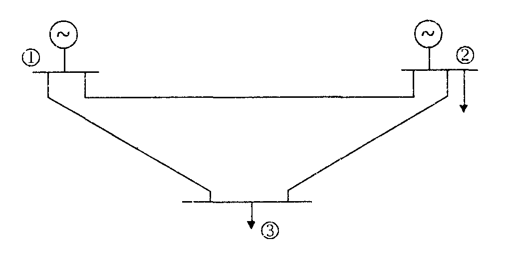
**Goal:** Minimize total generation cost while meeting total demand — the simplest form of *static* optimal control in power systems.
"""


# ╔═╡ ad8e9d79-e226-468e-9981-52b7cda7c955
md"""
### Quadratic Program (QP) Formulation of Economic Dispatch

Economic dispatch can be formulated as a **quadratic program**, where generation cost is convex and constraints balance supply and demand conditions.

```math
\begin{align}
\min_{p_g} \quad & \sum_{g \in \mathcal{G}} C_g(p_g) \\
\text{s.t.} \quad & \sum_{g \in \mathcal{G}} p_g = \sum_{d \in \mathcal{D}} P_d \quad \text{(power balance)} \\
& p_g^{\min} \le p_g \le p_g^{\max}, \quad \forall g \in \mathcal{G} \quad \text{(capacity limits)}
\end{align}



where:

| Symbol        | Description                                            |
|:------------- |:-------------------------------------------------------|
| $p_g$         | power output of generator $g$                          |
| $C_g(p_g)$    | cost function of generator $g$ (often quadratic: $a_g p_g^2 + b_g p_g + c_g$) |
| $P_d$         | power demand at load $d$                               |
| $\mathcal{G}$ | set of generators                                      |
| $\mathcal{D}$ | set of loads                                           |
"""

# ╔═╡ fc329e51-e91c-4d83-b6fe-07a3bce44d5d
md"""
### Exercise: Formulate the ED Problem for the 3-Bus Network

**Task:**  
Apply the generic formulation to the 3-bus system. Identify:
1. The decision variables  
2. The objective function  
3. The power-balance constraint  
4. Generator bounds

> 💡 *Hint:* Treat each generator’s output as a controllable decision variable. The total generation must exactly match total load.
"""

# ╔═╡ d767175f-290d-403e-99de-d3a8f2ccb5b5
md"""
#### ED formulation for the 3-bus example

Here is the complete formulation for our 3-bus example:

```math
\begin{align}
\min_{p_1, p_2} \quad & 8p_1 + 2p_2 \\
\text{s.t.} \quad & p_1 + p_2 = 125 \quad \text{(power balance)} \\
& 0 \leq p_1 \leq 100 \quad \text{(Gen 1 limits)} \\
& 0 \leq p_2 \leq 40 \quad \text{(Gen 2 limits)}
\end{align}
```

**Solution:** $p_1$ = 85 MW, $p_2$ = 40 MW
- Total cost: 8*85 + 2*40 = 760\$/hour
- Gen 2 at maximum capacity (greedy)
- Gen 1 supplies remaining demand

> ⚙️ Control Interpretation: This is a static control allocation problem. In later sections, we’ll extend such formulations to time-varying states and control trajectories.
"""

# ╔═╡ c9d0e1f2-0894-4340-a18b-72f8e1204432
md"""
### Discussion

Reflect on the ED formulation:

- What type of optimization problem is this (linear, quadratic, convex)? 
- How does this formulation abstract away the **physical grid topology**? What kind of graph is it?
- What critical physics are missing if we care about **how** power moves through lines?

> 🧭 **Bridge to next topic:**  
> ED models the **steady-state optimization** problem without considering power flow through lines.
> The next step — **DC power flow** — adds physical coupling constraints between buses.
"""

# ╔═╡ 9d1ea9be-2d7b-4602-8a8e-8426ea31661a
md"""
### Why the Simplified Model Falls Short

The simple ED model ignores the **network physics** that govern actual power transfer:
- Power has **direction** — it flows through transmission lines governed by voltage phase angles so the graph needs to be directed.
- Each line has a **thermal rating**: excessive current causes heating, sagging, or even wildfires.
- What is a power line:
  - Metal coil that expands and heats up when current is high.

In real systems, exceeding thermal limits does not immediately stop power flow — it simply becomes unsafe, which requires branch flow constraints.
Thus, the next layer of realism is to introduce branch constraints → **DC power flow**.
"""

# ╔═╡ 71ba62e6-bcc1-4e9b-91cd-a8860ba0d2b5
md"""
## DC Power Flow

To make ED more realistic, we include the grid’s topology by adding branch constraints.
The **DC power flow model** provides a linearized approximation of AC power flow and enforce Kirchhoff’s laws.

**Parameters:**
- Line reactance $x_{ij}$
- Line limit $F_\ell^{\max}$
- Generator set $\mathcal{G}_i$ at bus $i$ (nodal generation)
- Load set $\mathcal{L}_i$ at bus $i$ (nodal load)
- Generator limits $P_j^{\min}, P_j^{\max}$
- Costs $C_j(P_j)$ quadratic or piecewise-linear for generator $j$

**Decision Variables:**
- Generator outputs $P_j$ for $j \in \mathcal{G}_i$
- Bus angles $\theta_i$ for $i \in \mathcal{N}$
- Line flows $f_\ell$ for $\ell \in \mathcal{L}$

> 🧩 We will see later that the bus angles $\theta_i$ enter as *state variables* in the control dynamics.
"""

# ╔═╡ 7b4800c2-133d-4793-95b1-a654a4f19558
md"""
### DC Power Flow Formulation

The DC power flow optimization problem combines economic dispatch with network physics:

```math
\begin{align}
\min_{P_j, \theta} \quad & \sum_{i \in \mathcal{N}} \sum_{j \in \mathcal{G}_i} C_j(P_j) \\
\text{s.t.} \quad & \sum_{j \in \mathcal{G}_i} P_j - \sum_{j \in \mathcal{L}_i} P_j = \sum_{k: (i,k) \in \mathcal{L}} \frac{1}{x_{ik}} (\theta_i - \theta_k) \quad \forall i \in \mathcal{N} \\
& f_\ell = \frac{1}{x_\ell} (\theta_{i(\ell)} - \theta_{j(\ell)}), \quad -F_\ell^{\max} \leq f_\ell \leq F_\ell^{\max} \quad \forall \ell \in \mathcal{L} \\
& P_j^{\min} \leq P_j \leq P_j^{\max} \quad \forall j \in \mathcal{G}_i, \forall i \in \mathcal{N} \\
& \theta_{\text{ref}} = 0
\end{align}
```

- Reactance of line $x_{ij}$. $\frac{1}{x_{ij}} = b_{ij}$: susceptance (manufacturer specified)
- Reference bus: only for modeling, you can pick any bus as the reference bus. We only care about angle differences (which carries current through lines
- Individual bus angle has no physical meaning
"""

# ╔═╡ 7961c1d1-3e82-49ea-8201-c5f82066d70d
md"""
### Exercise: Solve DCOPF (solver suggested: Ipopt)

Let's apply the DC power flow formulation to our 3-bus network with line constraints:

![3-Bus Network with Constraints](https://www.al-roomi.org/multimedia/Power_Flow/3BusSystem/SystemIII/Murty3BusSystem.jpg)

**How did I get the numbers:**
- Assume P1 generates 85 MW, with 50 MW of load, the net injection is 35 MW
- Assume P2 generates 40 MW, with no load, net injection is 40 MW (we take upwards arrow as injection)
- Bus 3 has no gen, only load
"""

# ╔═╡ 91b8a3e4-81ed-49fe-b785-4feacfd8788d
md"""
### DCOPF Solution

Consult lecture slides for the solution and detailed analysis.
"""

# ╔═╡ f72775b9-818c-4a9b-9b66-cfccd88e17ed
md"""
### Wrap Up

This section has introduced the fundamentals of static optimal power flow problems including economic dispatch and DC optimal power flow. Key takeaways:

- You will see that without thermal limits, optimal dispatch can overload lines
- Reference bus is arbitrarily picked by the solver.
- Real systems are AC (complex voltages/currents) -- much harder. This is just a lightweight intro so we can think about expressing real-world problems as optimization formulations without overburdening ourselves with AC physics, which we will see in transient stability section.
"""

# ╔═╡ 53ab9b31-78aa-49b6-9e24-df47aa80f25a
md"""
# Introduction to Transient Stability

While static optimization provides a foundation, real power systems are dynamic. When disturbances occur—faults, switching events, or sudden load changes—the system experiences transients before settling to a new equilibrium. Understanding and controlling these transients is essential for system stability.

## Transient Dynamics
"""

# ╔═╡ 1e337cdf-8add-42ab-a62f-23069e34ec39
md"""
## What are transients?

When current or voltage changes suddenly — switching, faults, lightning, equipment failures, etc. — the system experiences a **transient**

- Transients are short-lived, high-frequency events where stored magnetic and electric energy exchange rapidly.
- **Faraday's law** of electromagnetic induction governs these effects:

  A change in magnetic flux through a circuit induces a voltage across it.
  
  ```math
  v(t) = \frac{d\Phi(t)}{dt}
  ```
  
  where $\Phi(t)$ is the magnetic flux through the circuit.
"""

# ╔═╡ 23dc8fd4-59a1-414f-a165-b509458abd18
md"""
## Transients Continued

The relationship between flux and current leads us to the fundamental equations governing inductors:

- For an inductor, the magnetic flux $\Phi$ is proportional to the current:
  
  ```math
  \Phi(t) = L\,i(t)
  ```
  
  where $L$ is the inductance (magnetic energy stored per unit current).
  
- Substituting gives the familiar time-domain voltage rule:
  
  ```math
  \boxed{v_L(t) = L\,\frac{di(t)}{dt}}
  ```

Note that steady-state phasor analysis no longer holds due to the time-varying nature of the magnetic flux. I will draw the connection later.
"""

# ╔═╡ 5814ece5-51b3-4dba-953d-c1f4b6ab04a8
md"""
## Sinusoidal steady state

To connect time-domain transients with frequency-domain analysis, we assume all quantities have angular frequency $\omega$ to extract the phasors in steady-state. The current in time-domain is:

```math
\begin{align}
i(t) &= \operatorname{Re}\!\left\{ I\,e^{j\omega t} \right\},
\end{align}
```

Differentiate the current:

```math
\begin{align}
\frac{di(t)}{dt} &= \operatorname{Re}\!\left\{ j\omega I\, e^{j\omega t} \right\}.
\end{align}
```

Substitute into $v_L(t) = L\,\frac{di}{dt}$:

```math
\begin{align}
v_L(t) &= \operatorname{Re}\!\left\{ (j\omega L I)\, e^{j\omega t} \right\}.
\end{align}
```

## Phasor (frequency-domain) relation

We are now ready to extract the phasor representation of voltage. By definition, the **phasor** is the complex amplitude multiplying $e^{j\omega t}$.

From the previous expression,

```math
\begin{align}
v_L(t) &= \operatorname{Re}\!\left\{ (j\omega L I)\, e^{j\omega t} \right\},
\end{align}
```

the **voltage phasor** is

```math
\begin{align}
\boxed{V = j\omega L\, I}.
\end{align}
```
"""

# ╔═╡ c1d2e3f4-0894-4340-a18b-72f8e1204445
md"""
## Capacitor law: from time domain to phasor

Similar to inductors, capacitors also exhibit transient behavior. Let's derive the capacitor relationships:

A capacitor stores energy in an **electric field**. The stored charge $q(t)$ is proportional to voltage $v(t)$: 

```math
q(t) = C\,v(t)
``` where $C$ is the capacitance.

* The current is the rate of change of charge: 
```math
i_C(t) = \frac{dq(t)}{dt} = C\,\frac{dv(t)}{dt}
```

With $v(t)=\operatorname{Re}\{V e^{j\omega t}\}$,

```math
\begin{align}
\frac{dv(t)}{dt} &= \operatorname{Re}\!\left\{ j\omega V e^{j\omega t} \right\}, \\
i_C(t) &= \operatorname{Re}\!\left\{ (j\omega C V) e^{j\omega t} \right\}.
\end{align}
```

Hence, the **phasor relationship** is:

```math
\begin{align}
\boxed{I = j\omega C\,V}, \qquad
\boxed{Y_C = j\omega C}, \qquad
\boxed{Z_C = \frac{1}{j\omega C}}.
\end{align}
```
where $Y_C$ is the capacitive admittance and $Z_C$ is the capacitive impedance, and susceptance $B_C$ is imaginary part of $Y_C$.
The real part of $Y_C$ is conductance $G_C$, which is used in steady-state AC optimal power flow problems.
You could of course derive admittance and impedance for inductors following similar steps. The above steps connect the time-domain and phasor domain. Note that the above is for ideal inductors and capacitors.
"""

# ╔═╡ ca8dc9ed-0974-4205-9af4-a21c8a7cb707
md"""
## More realistic transmission line model

So far, we've considered circuit elements without considering their coordinates on the line. 
In real transmission lines, however, voltage $v(x,t)$ and current $i(x,t)$ vary **both** in time and along the line coordinate $x$.

Their spatial derivatives represent how these quantities change **per unit length:**

```math
\begin{align}
\frac{\partial v(x,t)}{\partial x} &\;\Rightarrow\; \text{voltage drop per unit length (V/m)}, \\
\frac{\partial i(x,t)}{\partial x} &\;\Rightarrow\; \text{current change per unit length (A/m)}.
\end{align}
```

**Real lines are lossy:**
- Conductor series resistance causes Ohmic losses (heat dissipation) in voltage $\Rightarrow$ adds $-R'\,i(x,t)$.
- Current leakage due to shunt conductance $\Rightarrow$ adds $-G'\,v(x,t)$.

Hence, the full **telegrapher's equations** are:

```math
\begin{align}
\frac{\partial v(x,t)}{\partial x} &= -L'\frac{\partial i(x,t)}{\partial t} - R'\,i(x,t),\\
\frac{\partial i(x,t)}{\partial x} &= -C'\frac{\partial v(x,t)}{\partial t} - G'\,v(x,t).
\end{align}
```
where $L'$ and $C'$ are the inductance and capacitance per unit length, and $R'$ and $G'$ are the resistance and conductance per unit length.
You can think about $R'$ and $G'$ as damping terms to account for losses and leakage. 
$L,C$ relate to energy storage, and $R,G$ relate to energy dissipation.
"""

# ╔═╡ 9716f6a5-54d6-4abc-b0df-82f5a30e0196
md"""
## How the above was derived

Consider a small line segment between $x$ and $x+dx$.
- Coordinate $x$ increases in the direction of current flow ($+x$).
- Current flowing in $+x$ direction: $i(x,t)$.
- Voltage between conductors (top to bottom) at position $x$: $v(x,t)$.

**1. Voltage change between segment ends:**

```math
v(x,t) - v(x+dx,t) = -\frac{\partial v(x,t)}{\partial x}\,dx.
```

**2. Series drops over $dx$:**

```math
\begin{align}
\text{Resistive drop} &:\; R'\,i(x,t)\,dx,\\
\text{Inductive drop} &:\; L'\,\frac{\partial i(x,t)}{\partial t}\,dx.
\end{align}
```

**3. Apply Kirchhoff Voltage Law:**

(The sum of voltage drops along the closed path must equal zero.)

```math
(R'\,i + L'\tfrac{\partial i}{\partial t})\,dx + \big[v(x+dx,t) - v(x,t)\big] = 0.
```

**4. Substitute and simplify:**

```math
\frac{\partial v(x,t)}{\partial x}\,dx = -L'\frac{\partial i(x,t)}{\partial t}\,dx - R'\,i(x,t)\,dx.
```

**5. Divide by $dx$:**

```math
\boxed{\frac{\partial v(x,t)}{\partial x} = -L'\frac{\partial i(x,t)}{\partial t} - R'i(x,t)}.
```

The negative sign indicates that voltage **drops** in the $+x$ direction due to both inductive ($L'\,\partial i/\partial t$) and resistive ($R'i$) effects.
"""

# ╔═╡ a5b6c7d8-0894-4340-a18b-72f8e1204451
md"""
# How does physics relate to optimization?

We now connect the time-domain physics to **Transient Stability–Constrained Optimal Power Flow (TSC-OPF)**, where the optimization must respect both steady-state **and** dynamic constraints after a disturbance.
"""

# ╔═╡ 34595bd9-874e-4ca9-bf3c-3ebef9a37cec
md"""
## TSCOPF formulation

```math
\begin{align*}
\min_{p,\,x(t),\,y(t)} \quad & C(p)  && \text{(1)}\\
\text{s.t.}\quad
& g_s(p) = 0 && \text{(2)}\\
& h_s^{-} \le h_s(p) \le h_s^{+} && \text{(3)}\\
& p^{-} \le p \le p^{+} && \text{(4)}\\[3pt]
& \dot{x} = f(x,y,p), \quad x(t_0)=I_x^0(p) && \text{(5)}\\
& 0 = g(x,y,p), \quad y(t_0)=I_y^0(p) && \text{(6)}\\
& h(x(t),y(t)) \le 0, \quad \forall t && \text{(7)}
\end{align*}
```

**Objective:** minimize operating cost or transmission losses. Eq. (2) includes steady-state nodal power balance constraints. Eq. (3) includes apparent/real power/reactive power/current flow constraints on lines. Eq. (4) includes generator capacity or voltage magnitude constraints.

> 📖 **Reference:** Abhyankar, S., Gross, G., Agrawal, A., & Malik, O. (2017). Solution techniques for transient stability-constrained optimal power flow. IET Generation, Transmission & Distribution, 11(12), 3075–3084. https://doi.org/10.1049/iet-gtd.2017.0345
"""

# ╔═╡ a9f00e8c-205e-45a9-83d4-1dea5b7627c1
md"""
## Dynamic Transient Constraints: (5)--(7)

The dynamic constraints (5)-(7) embed the time-parametrized physics of transient behavior into the optimization problem:

**Eq. (5):**
- State variables $x$ (rotor angles, speeds, control states). Initial states computed from steady-state solution corresponding to control variables $p$.
- System dynamics $f(x,y,p)$ — e.g., generator swing equations, Telegrapher equations, or capacitor/inductor transient models.
- Dependent variables $y$ (nodal voltages magnitude and angle, line currents, etc.).
- Control variables $p$ (generator setpoints, tap settings, shunt positions, etc.)
- Enforce the physics of transient after a disturbance.

**Eq. (6):** embed dynamics into steady-state constraints.
- The steady-state constraints $g(x,y,p)$ have same physical laws as (2) e.g. KCL but now must hold at every instant $t$'s states $x(t), y(t)$.

The final set of constraints ensures that the system remains within safe operating limits throughout the transient:

**(7) Transient limits:**

```math
h(x(t), y(t)) \le 0, \quad \forall t
```

- Enforce time-domain operating limits during the transient response.
- Examples:
  - Bus voltage magnitudes stay within limits.
  - Rotor angle differences remain stable.
  - Line thermal limits respected.
- Ensures **transient stability** under all time steps during disturbance.
"""

# ╔═╡ 22d5c113-82f0-4598-8c47-ead1face730e
md"""
## Solution Methods for TSC-OPF

Solving TSCOPF is computationally challenging due to the nonlinear nature of AC power and the embedded differential equations. Several approaches have been developed:

**Indirect (variational) Methods:**
- Based on Pontryagin's Maximum Principle.
- Replace the differential equations of dynamics with inequalities that approximate the behavior in steady-state by linearizing into additional static conditions.
- Examples: energy or Lyapunov functions or impose stability margin constraints on linearized Jacobian.

Instead of having to integrate over time, we get back a static nonlinear optimization problem that can be solved using standard solvers.

**In practice:**
- Mainly used for planning/screening/preventive security dispatch due to loss in accuracy.
- Not sufficient to guarantee transient stability under large disturbances.
- Validation still relies on time-domain (direct) simulation.
"""

# ╔═╡ 47e011b8-4fb8-4534-a504-ffe3009beb6e
md"""
## Direct Method: Simultaneous Discretization/Constraint Transcription

An approach that directly discretizes the differential equations. **Main idea:** Converts the time-dependent diff. eq. into a finite set of algebraic constraints before solving the optimization problem so transient stability simulator can be reused.

**Discretization approach:**
- The simulation horizon is divided into multiple time steps $t_0, t_1, \dots, t_N$.
- The diff. eq. is approximated at each step using numerical integration like implicit trapezoidal rule:

  ```math
  x(t) - \frac{\Delta t}{2} f(x(t), y(t), p)
  - x(t-\Delta t)
  - \frac{\Delta t}{2} f(x(t-\Delta t), y(t-\Delta t), p) = 0.
  ```

**Pros and Cons:**
- Produces one large-scale NLP that enforces the dynamics exactly for the entire trajectory (within discretization accuracy).
- Computationally demanding due to the high dimensionality of variables and constraints from discretization. Accurate gradients is expensive from trajectory sensitivity analysis. Hessians often approximated using BFGS updates.
"""

# ╔═╡ a3786b2d-9951-440f-854c-dfd40ad727f1
md"""
## Direct Method: Multiple Shooting

Multiple shooting offers a more numerically stable alternative to simultaneous discretization. It divides the simulation horizon into smaller time segments $[t_0,t_1], [t_1,t_2], \dots, [t_{N-1},t_N]$.

- Each segment starts from its own initial condition $x_i(t_i)$ and is integrated forward using the diff. eq. $\dot{x}=f(x,y,p),\, 0=g(x,y,p)$ to obtain the predicted final state $\hat{x}_i(t_{i+1})$.
- Constraint to ensure continuity between segments:

  ```math
  x_{i+1}(t_{i+1}) = \hat{x}_i(t_{i+1}),
  ```

Abstractly, the constraint form is:

```math
s_i = S_i(s_{i-1},p), \quad \forall i \in 1,\dots,N_S,
```

where $S_i(\cdot)$ is an implicit function that can be numerically integrated over segment $i$. This can be used for variables $x,y$.

**Pros:** Each segment can be integrated independently, so the Jacobian of the resulting NLP is better conditioned because the coupling is limited to segment boundaries instead of the entire trajectory. This segmentation improves numerical stability and allows for more efficient large-scale computation.
"""

# ╔═╡ c3d4e5f6-0894-4340-a18b-72f8e1204458
md"""
## Trajectory Sensitivity Analysis of TSC-OPF

Both direct methods require gradient information. Sensitivity analysis can provide this efficiently. 
**Purpose:** Quantify how system variables $x(t),y(t)$ changes with respect to small variations in control variables $p$ or initial conditions. 
Recall that with different control settings $p$, the entire transient trajectory changes and we would need to simulate the dynamics again to see the consequences.
This is expensive. Sensitivity analysis tells you how the trajectory and stability margins change with small variations in $p: \frac{\partial x}{\partial p}$ without running the full simulation for every small perturbation.

**Relation to numerical methods:**
- These sensitivities provide gradient information for solvers, which is used for both multiple shooting and constraint transcription.
"""

# ╔═╡ 946ad231-4ddf-43a3-b2b9-95d502f4b5e9
md"""
## Forward Sensitivity Method

The forward sensitivity method computes gradients by integrating sensitivity equations forward in time:

- Perform a forward integration of the sensitivity equations alongside the original diff. eq. system.
- Efficient when the number of parameters is small.
- The computational complexity is $\mathcal{O}(n_p)$, since $n_p$ forward integrations are required to compute the sensitivities.

**Formulation:**

For the original diff. eq. system:

```math
F(\dot{x}(t),\, x(t),\, p) = 0.
```

The corresponding variational diff. eq. for the sensitivities is:

```math
\frac{\partial F}{\partial \dot{x}}\,\dot{s}
+ \frac{\partial F}{\partial x}\,s
+ \frac{\partial F}{\partial p} = 0,
```

with initial condition

```math
s(t_0) = \frac{\partial x(t_0)}{\partial p}.
```

- Each parameter $p_i$ perturbs the system differently.
- Forward method tracks this by integrating a new "copy" of the linearized system, which shares the same Jacobian (including state dynamics and algebraic equations of KCL etc.) as the original differential equations.

**Pros and cons:**
- **Pros:** Simple to implement, accurate efficient when number of parameters is small.
- **Cons:** Computational cost grows linearly with number of parameters.
"""

# ╔═╡ f6399741-9b5f-4bd3-bae7-6cc1ed1bd718
md"""
## Adjoint Method

When the number of parameters is large, the forward method becomes expensive. The adjoint method is an alternative that only needs one backward integration in time to compute the sensitivities.

**Formulation:**

- Consider 

  ```math
  G(p) = \int_{t_0}^{T} g(x, p)\,dt.
  ```

- We want the gradient given by:

  ```math
  \frac{\partial G}{\partial p}
  =
  \int_{t_0}^{T}
  \left(
  \frac{\partial g}{\partial p}
  - \lambda^{\mathsf{T}} \frac{\partial F}{\partial p}
  \right) dt,
  ```

- The adjoint multiplier $\lambda(t)$ satisfies

  ```math
  \dot{\lambda}
  =
  -\,\frac{\partial g}{\partial x}
  + \lambda^{\mathsf{T}}\frac{\partial F}{\partial x}.
  ```

  where $\lambda(T)=0$.

**Pros:**
- Efficient when the number of parameters is large.
- The gradient is obtained in one backward integration.

**Cons:**
- Higher memory cost due to storage of trajectory data and state variables in backward integration.

One can also obtain the gradients by finite differences, which is based on truncated Taylor series expansion.
"""

# ╔═╡ 214eacc5-0b60-44b8-8a53-9cce369debdd
md"""
# Power System History and Modern Power System

To understand why transient stability matters today, we must go back to see how power systems have evolved. The grid's dynamic behavior has fundamentally changed with the integration of renewable energy.

## The Fuel Era (20th Century)

Electricity produced mostly by coal, gas, nuclear. Generators are large synchronous machines with big spinning masses. Stable and predictable. Inertia from these machines naturally provides flexibility in frequency stability. Grid ran reliably for decades.

## The Renewable Era (2000s--Today)

Wind expanded in 2000s, solar PV took off after 2010. Renewables now more than 20--40% of real-time demand in some regions; dynamics changed.
"""

# ╔═╡ a7b8c9d0-0894-4340-a18b-72f8e1204464
md"""
## Synchronous Generators: How electricity is generated

![Generator Cross-Section](https://www.electricaltechnology.org/wp-content/uploads/2022/09/Cylindrical-Alternator-or-Synchronous-Generator.png)

- Rotor (heavy spinning mass) driven by turbines (steam, gas, hydro)
- Faraday's law: changing magnetic field induces voltage in stator
- Called "synchronous" because the rotor spins in sync with the grid's frequency (50 Hz in Europe, 60 Hz in North America)
- If the grid frequency is 60 Hz, the rotor turns at a speed locked to 60 Hz
"""

# ╔═╡ 6b64a495-6039-408c-91a9-4dfddf21d857
md"""
## Spinning Mass in a Generator

- Inside a synchronous generator is a rotor — basically a giant heavy wheel of steel and copper (tens or hundreds of tons)
- Turbines (steam from coal/nuclear, gas combustion, or flowing water in hydro) push on the rotor to make it spin
- That rotor's mechanical rotation creates a rotating magnetic field, according to Faraday's law of induction, a changing magnetic field induces an alternating voltage in the stator windings
- This is why the system is predictable: we know how to control these rotors. Put in more fuel to generate more power
"""

# ╔═╡ b5159081-3b0a-459a-9c5b-c2b4911d79e2
md"""
## Generator Frequency Formula

**Frequency Formula:**

```math
f = \frac{N \times \text{RPM}}{120}
```

where $N$ = number of poles, RPM = rotor speed

**Examples:**
- 2 poles, 3600 RPM → 60 Hz
- 4 poles, 1800 RPM → 60 Hz

**Why 50/60 Hz?** Historical choices: early engineers (Westinghouse, Edison, etc.) picked values that balanced motor performance and generator design. Once infrastructure was built, it became a standard.
"""

# ╔═╡ ad22ab28-884e-4c3b-8265-51a44685343d
md"""
## Kinetic Energy

**The rotor has stored kinetic energy:**

```math
E_{\text{kinetic}} = \frac{1}{2} J \omega^2
```

where $J$ = moment of inertia (depends on mass + geometry), $\omega$ = rotor speed

**If demand suddenly exceeds supply (a generator trips):**
- That small slow down of a rotor releases some of its stored kinetic energy into the grid instantly
- But because there are so many large spinning machines, the grid behaves like a conveyor belt with so many wheels tied together. If one slows a bit, the others share the imbalance, so frequency changes slowly because the system has a huge inertia
- This gives time for operators to fix things
- Even if there are imbalances, things wouldn't get out of hand fast since there are so many other generators. They can share the load so each only needs to spin a little faster to keep up the frequency
"""

# ╔═╡ 01ebbe37-0681-47bb-b851-5f16b9f4aeb5
md"""
## Inverters - Renewables

The modern power grid faces new challenges with the integration of renewable energy sources. **Today, renewables supply 20–40\%+ of real-time demand.**

Cleaner, cheaper, more sustainable — but dynamics changed.

Most renewables (solar PV, modern wind turbines, batteries) produce DC electricity (direct current).

**What's the problem of DC power?**
- It only has amplitude (magnitude of voltage/current)
- No phase, no frequency
- But recall AC current has the waveform (that's why we have leading/lagging current which controls reactive power and power factor correction)
- We need amplitude, frequency, and phase to describe AC current
- That's why we need inverters, power electronics device that synthesizes sinusoidal AC from DC
"""

# ╔═╡ 86d07665-753e-4dbe-aa84-5b23ec0a616f
md"""
## Inverter Operation

**How it operates?**

1. Takes DC input from solar panels, wind turbine
2. Use power electronics that switches thousands of time per second to synthesize an AC waveform
3. Note that even the output is a smooth sinusoidal AC waveform, inside the inverter the switches turn the DC voltage on and off thousands of times per second (typical switching frequency = 2–20 kHz, sometimes higher) to approximate that smooth waveform
4. So even though the output is continuous, it's created by on/off pulses internally
5. The inverter synchronizes the AC output to the grid's frequency and phase. If grid is 60 Hz → inverter outputs 60 Hz. If grid is 59.9 Hz (after a disturbance) → inverter follows 59.9 Hz.
6. The voltage, current, and power factor are controlled through the programmed algorithms
"""

# ╔═╡ 8e4dc912-14ff-4290-8f96-926493e5ef81
md"""
## Inverter Control Modes

**In summary, the inverters are programmable devices by operators with control algorithms to act like generators. They wait for a signal from a grid so they can be:**

- **Grid-following:** track the grid's voltage and frequency → inject current accordingly
- **Grid-forming:** behave like a voltage source, set their own frequency/voltage reference, and to adjust for power imbalance (some research area I heard of)

They are not really generators - no spinning mass, no inertia, but they use control algorithms to mimic generator behavior.
"""

# ╔═╡ c5d6e7f8-0894-4340-a18b-72f8e1204471
md"""
## Internal View of Inverters

![Internal View of Inverter](https://upload.wikimedia.org/wikipedia/commons/thumb/e/ee/Sunny_Boy_3000.jpg/1200px-Sunny_Boy_3000.jpg)

- Capacitors and switching components on electronic mainboards (like in computer's motherboard, blue cylinders in upper left corner of the picture)
- Programmable behavior defined by control firmware
"""

# ╔═╡ c0cc1b94-e651-40c2-8084-e9ebfad2a457
md"""
## Problems with Inverters

**This is all software-based. You do not have a natural physical property like a spinning rotor and inertia.**

- No big spinning mass directly tied to frequency, so frequency changes much faster after a disturbance
- The device measures grid signal and forces its output to follow
- Unless explicitly programmed, they don't know when the conveyor belt slows down or speeds up (recall the previous analogy)
- Even if they do, they don't have the capacity like big generators
- **This is the key part:** they are just switching circuits with no agency to ramp up the power output (nature of renewables is their output is often independent of human control). Output is limited by weather and energy availability (sun/wind).
- Renewables also locate in remote areas with long transmission lines, and the nature of their unpredictability (weather), makes their generation highly uncertain

**We will build up to inverter control after we cover the generator swing equations.**
"""

# ╔═╡ 4702e992-a163-40f3-ab55-f9e8e848d0c7
md"""
# Generator Swing Equations

The generator swing equations are the cornerstone of power system dynamics. They describe how generators respond to power imbalances, connecting mechanical and electrical power through rotational forces.

## Newton's Second Law

We begin with the fundamental physics. **Linear Version:**

```math
F = ma
```

where $F$ = force (N), $m$ = mass (kg), $a$ = acceleration (m/s²)

This says: imbalance of forces → acceleration of mass.

**Rotational Version:**

For a rotating body (like a generator rotor), the equation is:

```math
T = J\alpha
```

where $T$ = torque (N·m), $J$ = moment of inertia (kg·m²), the rotational mass. $\alpha$ = angular acceleration (rad/s²)

This says: imbalance of torques → rotor accelerates or decelerates.

Think torque as the angular equivalent of force.
"""

# ╔═╡ 1566dce2-fd36-4110-8220-97eefe043cbb
md"""
## Applied to Generator Dynamics

Now we apply Newton's second law to a generator rotor. **There are two main torques acting on a synchronous generator's rotor:**

- Mechanical torque from the turbine (steam, gas, water) pushing the rotor: $T_m$
- Electromagnetic torque from the stator's magnetic field resisting the rotor (this is the grid "pulling" power out): $T_e$

**Torque imbalance:**

```math
J\alpha = T_m - T_e
```

where $\omega$: angular speed of rotor (rad/s), $\alpha = \dot{\omega}$: angular acceleration (rad/s²)

**If $T_m > T_e$:** rotor accelerates

**If $T_m < T_e$:** rotor slows down

**If equal:** steady rotation
"""

# ╔═╡ 9bd48789-5d3d-495c-acd3-6586ae616136
md"""
## From Torque to Power

To connect torque dynamics with electrical power, we relate rotational motion to power. Recall $P = Fv$ (mechanical power is generated by a force $F$ on a body moving at a velocity $v$). In rotational systems, power is related by torque and angular speed (you can think about it as rotational equivalent as force)

**Power = torque × speed:**

```math
P = T \cdot \omega
```

So:
- Mechanical power input: $P_m = T_m \cdot \omega$
- Electrical power output: $P_e = T_e \cdot \omega$

Multiply the torque balance by $\omega$:

```math
J\omega\dot{\omega} = P_m - P_e
```

This relates how fast the mass is spinning ($\omega$) to the imbalance of power input (generation) and power withdrawal (load + losses).

In practice, generators operate close to system frequency, so the generators spin at an angular velocity that is close to that 60 Hz constant. Since the variations are mostly tiny, we can define inertia constant $M = J\omega$

And we get the generator swing equation:

```math
M\dot{\omega} = P_m - P_e
```

**Interpretation:**
- Inertia constant $M$, measures how much the rotor resists speed change (bigger mass → slower frequency drift)
- Mechanical input power (from fuel, water, steam): $P_m$
- Electrical output power delivered to the grid: $P_e$
"""

# ╔═╡ a9b0c1d2-0894-4340-a18b-72f8e1204477
md"""
## Per-Unit Generator Swing Equation

**Per-unit versions:**

Power are often defined at per unit, so we have:

```math
\frac{J\omega_s}{S_{\text{base}}} \dot{\omega} = (P_m - P_e)_{\text{pu}}
```

There are sources that define $H = \frac{1}{2}\frac{J\omega_s^2}{S_{\text{base}}} \Rightarrow \frac{2H}{\omega_s} = \frac{J\omega_s}{S_{\text{base}}}$

$H \triangleq \frac{E_k}{S_{\text{base}}} = \frac{\frac{1}{2}J\omega_s^2}{S_{\text{base}}}$ comes from kinetic energy

So we have per unit swing:

```math
\frac{2H}{\omega_s} \dot{\omega} = (P_m - P_e)_{\text{pu}}
```
"""

# ╔═╡ abcd31d0-c6eb-4bc7-a752-83a8d7f6fda1
md"""
## Damping and Another Form of Generator Swing Equations

Some also add damping:

```math
M\dot{\omega} + D(\omega - \omega_s) = P_m - P_e
```

as penalties to frequency deviation. $D$ captures any restoring force, or frictions and losses

We can also write the per-unit acceleration form:

```math
2H \dot{\omega}_{\text{pu}} = (P_m - P_e)_{\text{pu}}
```
"""

# ╔═╡ b16732b7-ec08-43c7-9c08-489c8c8bbecb
md"""
## Why This Matters

- Stability depends on balancing generation and demand
- Inertia slows down changes in frequency, buying time for control actions

**Power imbalance effects:**
- If $P_m > P_e$: extra power → rotor speeds up → frequency rises
- If $P_m < P_e$: shortage → rotor slows → frequency falls

**Inertia $M$ slows down how fast this happens.**
- With many generators, $M$ is big. For a given imbalance, frequency drifts slowly → grid is flexible
- With fewer machines (more renewables), $M$ is smaller → frequency changes faster → grid is fragile

This is shown by writing the equation as $\dot{\omega} = \frac{P_m - P_e}{M}$. For a big $M$, the angular acceleration (frequency) is smaller when there is an imbalance.
"""

# ╔═╡ 8ee16365-6d48-4073-9482-44dd58b7e338
md"""
## How Does It Relate to Inverters?

The swing equation framework extends beyond traditional generators. We previously discussed grid-following inverters.

**Its control law works as:**

1. Measure voltage and frequency of the grid
2. Gets desired power output from an operator or solved from a market
3. Adjust its AC current output to deliver the desired power output at voltage and frequency GIVEN by the grid

The problem is it has no control over other parameters like voltage and frequency. The power output is only stable if the rest of the grid maintains a good reference.
"""

# ╔═╡ f05940b2-5a30-46dc-8811-5f3d6b0c74a0
md"""
## Grid-forming Inverters

Grid-forming inverters represent a more advanced control paradigm that enables renewables to provide grid support:

- It behaves as controlled voltage source that defines its own reference voltage and frequency
- Let the frequency shift slightly to reflect power imbalance between the renewable generation and the rest of the grid, so other machines (generators) know to ramp up or down
- Able to define its own frequency is the key for the renewable to behave like a synchronous generator, and we now have the ability to model it in a swing equation by giving it a virtual mass defined by the local frequency

We can now emulate synchronous machine behavior via controlling the "virtual inertia".

> 📖 **Reference:** J. Driesen and K. Visscher, "Virtual synchronous generators," 2008 IEEE Power and Energy Society General Meeting - Conversion and Delivery of Electrical Energy in the 21st Century, Pittsburgh, PA, USA, 2008, pp. 1-3.
"""

# ╔═╡ 75deac76-f89c-4b84-a132-67591177f5dd
md"""
## Virtual Inertia Law in Grid-Forming Inverter

**Physics is replaced by software:**

```math
M_{\text{virtual}} \dot{\omega} = P_{\text{ref}} - P
```

**Parameters:**
- Tunable parameter by the controller $M_{\text{virtual}}$, chosen to represent how fast the inverter responds to frequency changes
- Recall $M = J\omega$. Since we have no physical inertia $J$, the virtual mass is just a modeling choice
- Reference active power dispatch (from operator): $P_{\text{ref}}$
- Measured actual active power delivered: $P$
- Inverter's internal frequency reference value: $\omega$

**Effect of $M_{\text{virtual}}$:**
- A larger $M_{\text{virtual}}$ means the inverter allows its frequency to drift slower, a "heavier" machine
- A smaller $M_{\text{virtual}}$ means the inverter reacts more quickly, a "lighter" machine
"""

# ╔═╡ 0a2c4c0a-c68e-4f21-afbb-1b80791ec166
md"""
## Virtual Inertia

**How it works:**
- The inverter adjusts its internal frequency reference according to power imbalance
- That frequency reference drives its voltage output, which the grid "sees"
- To the rest of the system, this looks just like a synchronous machine rotor slowing/speeding under imbalance

- There's no heavy rotor. It emulates the inertia behavior of synchronous machines through software control.
- But this is not sustained. It can only hold it until the renewable saturates, which is less than a second since they don't have as much buffer as traditional generators.
- Other problems: semiconductor ratings, thermal limits, hard to tune $M_{\text{virtual}}$, cost, legacy devices, etc.

**Why this is such a big deal:** renewables can now respond to a grid-wide drop in frequency because it can behave almost like a synchronous generator through control law

## Demo of swing equation / virtual inertia response:
- When there's a positive power imbalance, the frequency will increase.
- Larger inertia slows down the rate at which frequency rises. This shows up as a curve that rises more gently (less sharply concave) because a heavier system resists acceleration more.
- Increasing damping reduces the steady-state frequency deviation for a given imbalance and allows the system to settle faster. Higher damping provides a stronger corrective force that pulls frequency back toward nominal. 
- In the plot, we will see it makes the plot level off sooner.
"""

# ╔═╡ e14c2b45-3a7d-4e27-9c13-79ae514b1881
@bind M Slider(0.5:0.5:10.0, default=5.0, show_value=true)

# ╔═╡ 6ff3fd90-23cd-4cd0-95cf-d4e1d5ac3bdf
@bind D Slider(0.0:0.1:5.0, default=1.0, show_value=true)

# ╔═╡ b32a299d-4d0a-4e8b-b576-15bb32acad24
@bind ΔP Slider(-0.5:0.05:0.5, default=0.2, show_value=true)

# ╔═╡ 4db9cfa4-66c7-4b71-b0b3-5c16eaa2bb9e
md"""
### Interactive: Swing Equation / Virtual Inertia Response

Use the sliders above to adjust:

- **M** — inertia (or virtual inertia)  
- **D** — damping  
- **ΔP** — power imbalance (positive = deficit in electrical power, negative = surplus)

The plot shows the **frequency deviation** response over time.
"""

# ╔═╡ a0b43f28-8e17-4633-8eab-b9554e05c8f6
begin
    # Nonlinear swing-like ODE: M * dω/dt + D*ω = ΔP
    function swing!(dω, ω, p, t)
        M, D, ΔP = p
        dω[1] = (ΔP - D*ω[1]) / M
    end

    ω0 = [0.0]  # initial frequency deviation
    p = (M, D, ΔP)
    tspan = (0.0, 10.0)

    prob = ODEProblem(swing!, ω0, tspan, p)
    sol  = solve(prob, Tsit5())

    plot(sol.t, [u[1] for u in sol.u],
        xlabel = "Time (s)",
        ylabel = "Frequency deviation",
        title  = "Generator Swing / Virtual Inertia Frequency Response",
        legend = false)
end


# ╔═╡ c7d8e9f0-0894-4340-a18b-72f8e1204484
md"""
## Grid-following inverters - Droop Control

Droop control enables automatic power sharing among generators and inverters: generators naturally slow down if overloaded, resulting in a drop in frequency (droop). Droop control allows each generator to increase its power output in response, but in proportion to its droop coefficient, so that all generators share the load change fairly.

Grid-forming inverters are programmed with droop control:

```math
P = P_{\text{set}} - \frac{1}{K_p} (\omega - \omega_0)
```

where $\omega_0$: nominal frequency, $P_{\text{set}}$: reference power output, $K_p$: droop constant (rad/s per MW or Hz per MW) telling inverter how much to adjust power output when frequency changes. Hence when frequency drops, power will rise.

Overload leads to frequency drop, and power will rise according to the relationship. If frequency rises, power will decrease to maintain the frequency.
"""

# ╔═╡ 20d5d03f-0225-4d3c-b0d2-d7440340b821
md"""
## Reactive Power and Voltage Control (Q-V Droop)

Just as frequency droop controls active power balance, voltage droop controls reactive power balance. Analogous for voltage support:

```math
V = V_0 - K_q (Q - Q_{\text{set}})
```

or

```math
Q = Q_{\text{set}} - \frac{1}{K_q} (V - V_0)
```

If reactive demand $\uparrow$ (voltage dips), generator/inverter increases reactive power injection.

**Two important components of stability:** frequency and voltage. If there are deviations, adjust active and reactive power accordingly

- Interpretation of $1/K_p$ = MW per Hz: "How much active power do I add if frequency drops by 0.1 Hz?"
- Interpretation of $1/K_q$ = Mvar per V → "How much reactive power do I add if voltage drops by 0.01 pu?"

## Summary: Generator and Inverter Dynamics

Synchronous generators naturally provide inertia and adjust their output through physical dynamics, giving the grid its inherent frequency stability.
Inverters lack this physical behavior, so control algorithms such as virtual inertia and droop control are introduced to let them share changes in load and maintain frequency and voltage—just as generators have always done. 
Droop control is essential because it enables multiple devices to automatically coordinate their power output. With generator and inverter dynamics in place, we now turn to **dynamic load models**, which describe how electricity demand behaves during disturbances.
"""

# ╔═╡ 37f242b9-454f-4361-a2e1-98acae57b6fe
md"""
# Dynamic Load Models

So far, we've focused on generation dynamics. However, loads also exhibit dynamic behavior that significantly impacts system stability. Understanding how loads respond to voltage and frequency changes is crucial for accurate transient analysis.

## Dynamic Load Models
"""

# ╔═╡ 4211a2c2-4a3a-4a63-8d2e-dc6c94e0cfc6
md"""
## Steady-State Load Models in ACOPF/DCOPF

We begin by reviewing how loads are typically modeled in static optimization. In optimal power flow (OPF), all quantities are **time-invariant**. $\dot{x} = 0$, time parameter $t$ does not appear in the equations.

At each load bus:

```math
P_D = \text{fixed real power demand}, \qquad
Q_D = \text{fixed reactive demand}.
```

These loads can be either:
- Constant power: $P_D, Q_D$ are specified numerical values; or
- Voltage-dependent (ZIP) as motors draw different amount current to maintain torque:

  ```math
  P(V) = P_0 (a_P V^2 + b_P V + c_P), \quad
  Q(V) = Q_0 (a_Q V^2 + b_Q V + c_Q).
  ```

Power-flow balance:

```math
P_G - P_D = \text{network losses}, \qquad
Q_G - Q_D = 0.
```

However, the static load model has important limitations. Interpretation of the above model:
- Loads are fixed regardless of system conditions, or at most respond to nodal voltage.
- No memory or dynamics -- they change only between static operating points.
- The OPF represents a single equilibrium snapshot of the system.

**Next:** Dynamic models generalize this by letting $P_D$ and $Q_D$ **evolve over time** with voltage and frequency. The grid's sink can be dynamic too even though we tend to think about it as a fixed parameter.
"""

# ╔═╡ 8ca0ad91-2fb5-4e64-9f6f-5498fa39d44b
md"""
## Dynamic Load Models - Induction Motor Model

Dynamic load models capture the time-dependent response of loads to system disturbances. In dynamic load models, the active and reactive power is represented as a function of the past and present voltage magnitude and frequency of the load bus. This type of model is commonly derived from the equivalent circuit of an induction motor.

Most real-world loads (fans, pumps, compressors) are induction motors.

Their active/reactive power do not change instantaneously with voltage change but rather dynamically by changing the motor's rotor speed $\omega_r$ to maintain torque. Hence, the power consumption depends on both voltage and frequency.

```math
P_d = f_P(V, \omega_r), \qquad Q_d = f_Q(V, \omega_r),
```

so the load has internal dynamics, unlike static $P_D, Q_D$ in ACOPF.
"""

# ╔═╡ a1b2c3d4-0894-4340-a18b-72f8e1204490
md"""
## Rotor Dynamics

The key parameter describing induction motor operation is slip, which relates rotor speed to synchronous speed:

**Slip:**

```math
s = \frac{\omega_s - \omega_r}{\omega_s},
```

where
- Synchronous electrical speed is $\omega_s$ (given by $2\pi f_s$), set by system frequency,
- Mechanical rotor speed (frequency at the load): $\omega_r$

**Operating regions:**
- When rotor is synchronous with system frequency: $s = 0$ $\rightarrow$ no induced torque.
- Normal operation: $0 < s < 1$. Rotor is slightly slower than the rotating field $\rightarrow$ induces current $\rightarrow$ produces torque.
- Stall: $s \to 1$. Rotor stopped, max current, high losses.

**Mechanical dynamics (sign flip if you differentiate w.r.t. slip):**

```math
J\frac{d\omega_r}{dt} = T_e(V,\omega_r) - T_m
\quad\Longleftrightarrow\quad
J\,\omega_s\,\frac{ds}{dt} = T_m - T_e(V,s).
```

**Variable definitions:**
- Rotor inertia (kg·$m^2$): $J$
- Rotor mechanical speed/frequency (rad/s): $\omega_r$
- Electromagnetic torque: $T_e$ (depends on bus voltage $V$, frequency $\omega_s$ (slip formulation), or $\omega_r$ (standard formulation)),
- Mechanical load torque: $T_m$
"""

# ╔═╡ 160fd7d9-a3c2-4f22-951e-deed6f32e09b
md"""
## Example: Induction Motor Response During a Voltage Sag

**Sequence of events:**

1. **Voltage drop:** $V$ suddenly decreases.
2. **Torque imbalance:** Electromagnetic torque $T_e(V,\omega_r)$ falls below mechanical torque $T_m$.
3. **Rotor slowdown:** $\omega_r$ decreases $\Rightarrow$ slip $s$ increases.
4. **Increased current and VAR demand:** The motor draws more current to restore torque, which further depresses voltage.
5. **Possible stalling:** If $V$ remains low, the motor stalls — reactive power skyrockets $\Rightarrow$ voltage collapse.

IM Modeling is key to capture this nonlinear instability mechanism.
"""

# ╔═╡ 56b58c9f-f8ce-4117-8105-70083c23fde9
md"""
## How TSC-OPF Prevents Motor Stalling and Voltage Collapse

The transient stability-constrained optimization framework directly addresses these instability mechanisms. **In TSC-OPF, dynamics and limits are enforced directly:**

```math
\dot{x} = f(x, y, p), \qquad 0 = g(x, y, p), \qquad h(x(t), y(t)) \le 0, \;\forall t.
```

**The IM model contributes to the dynamic states $x$ in TSC-OPF:**
- Induction motor slip $s$, generator rotor angles, inverter controls, etc.
- Their evolution $f(x,y,p)$ describes how voltages and speeds change after a disturbance.
- Dynamic constraints ensure stall condition is not reached.

**Constraint function $h(x(t),y(t))$:**
- Enforces time-domain limits such as

  ```math
  V_i(t) \ge V_{\min}, \quad \forall t \in [0, T_{\text{rec}}],
  ```

  where $T_{\text{rec}}$ is the recovery time. This ensures bus voltages remain within safe recovery bounds during the entire horizon after a disturbance.
- Prevents continued voltage sag that would drive $T_e(V,s)$ down and cause stalling.
"""

# ╔═╡ 03d81d40-f285-47d6-bbf4-db3e8efc7bd1
md"""
## Wrap up (Induction Motor Models)

Controls $p$ are chosen so that $f$ remains stable under disturbances, and the chain of events above is prevented since motor and network dynamics are embedded in $f$, $g$, and $h$.

This model is typically used when there's a fast transient or stalling, and the time scale is in milliseconds to second. Useful for short-term voltage stability and transient studies.
"""

# ╔═╡ a4b027e0-15e6-4097-acc9-358fb075fd7f
md"""
## Exponential Recovery Load (ERL): Motivation and Concept

Beyond individual motor dynamics, aggregate load behavior exhibits exponential recovery patterns. **Goal:** Represent aggregate load behavior during voltage recovery after a disturbance.

**Empirical Observation:**
- When voltage dips, total active and reactive loads drop immediately.
- Loads such as motor controls and HVAC systems **slowly restore** their power draw as voltage recovers.
- The recovery follows an **exponential time pattern**, not an instantaneous jump.

**Idea:**

Introduce internal states that describe this gradual return:

```math
P_d(t) = f_P(V(t),x_p(t)), \qquad Q_d(t) = f_Q(V(t),x_q(t)).
```

where $x_p(t)$ and $x_q(t)$ are the internal states of the active and reactive load.

These states evolve according to first-order differential equations, capturing the "memory" of how far the load has recovered.
"""

# ╔═╡ e93c6dc1-2f8d-4e2f-bbed-db926643f32a
md"""
## Adaptive Exponential Recovery Load (ERL) Model

The adaptive ERL model captures voltage-dependent recovery through differential equations. **Mathematical Form:**

```math
\begin{aligned}
T_p \frac{dx_p}{dt} &= -x_p\!\left(\frac{V}{V_0}\right)^{N_{ps}}
                   + P_0\!\left(\frac{V}{V_0}\right)^{N_{pt}},\\[3pt]
P_d &= x_p\!\left(\frac{V}{V_0}\right)^{N_{pt}},\\[6pt]
T_q \frac{dx_q}{dt} &= -x_q\!\left(\frac{V}{V_0}\right)^{N_{qs}}
                   + Q_0\!\left(\frac{V}{V_0}\right)^{N_{qt}},\\[3pt]
Q_d &= x_q\!\left(\frac{V}{V_0}\right)^{N_{qt}}.
\end{aligned}
```

**Parameters:**
- Internal recovery states (how much of the load has recovered): $x_p, x_q$
- Time constants (larger values $\Rightarrow$ slower recovery): $T_p, T_q$
- Nominal power withdrawals at reference voltage $V_0$: $P_0, Q_0$
- Transient exponents (immediate voltage sensitivity): $N_{pt}, N_{qt}$. How sharply load power reacts immediately when voltage changes (the short-term dip).
- Steady-state exponents (long-term voltage dependence): $N_{ps}, N_{qs}$. How much the load power changes in the long term after voltage settles to a new level.

**Interpretation:**
- After a voltage dip, power first follows the transient curve, then recovers exponentially toward the steady-state curve.
- When $V$ is weak, the recovery term $(V/V_0)^{N_{ps}}$ slows the rate of change — recovery stalls under low voltage.
- Recovery speed and power response both scale with voltage and almost halts under deep voltage sag.
"""

# ╔═╡ 3f7130a0-51d6-4493-b07e-e5bf178ce834
md"""
## Standard vs. Adaptive ERL Models

**Standard ERL model:**

```math
\begin{aligned}
T_p \frac{dx_p}{dt} &= -x_p + P_0\!\left[\!\left(\frac{V}{V_0}\right)^{N_{ps}} - \left(\frac{V}{V_0}\right)^{N_{pt}}\!\right],\\
P_d &= x_p + P_0\!\left(\frac{V}{V_0}\right)^{N_{pt}}.
\end{aligned}
```

**Key difference:**
- In the **standard** model, $dx_p/dt$ depends on $V$ only through the voltage-dependent driving term. The state $x_p$ recovers constantly—independent of voltage.
- In the **adaptive** model, recovery slows when $V$ is low: the term $(V/V_0)^{N_{ps}}$ reduces the rate of change. The two differ in how strongly the voltage affects recovery speed back to pre-disturbance load.

**Physical interpretation:**
- Standard ERL: suitable for moderate voltage dips.
- Adaptive ERL: more realistic for deep voltage sags.
"""

# ╔═╡ 18207180-a40b-4bb7-87bb-9a0752286cea
md"""
## ERL Parameters

- Parameters $(T_p, T_q, N_{ps}, N_{pt}, N_{qs}, N_{qt})$ are fitted empirically from from measurements of load recovery after voltage disturbances.
- They are not linked to physical machine constants, but to observed aggregate behavior of customer loads.

**Compared to IM Model:**
- Models **voltage-driven recovery** of active/reactive power demand, not frequency-driven mechanical motion.
- Represents the slower phase of system response (seconds to minutes) vs. fast electromechanical transients.

**Steady-state check:**

Setting $\dot{x}_p=\dot{x}_q=0$ gives $P_d=P_0(V/V_0)^{N_{ps}}$, $Q_d=Q_0(V/V_0)^{N_{qs}}$, so ERL naturally reduces to a static voltage-dependent load, showing that when dynamics died out, the model reduces to a steady-state load.
"""

# ╔═╡ 4d6fd1e2-9457-4f4c-84b1-62958a8b49de
md"""
## ERL in TSC-OPF and Contrast with Induction Motor Model

**TSC-OPF representation:**

```math
\dot{x} = f(x,y,p), \qquad 0 = g(x,y,p), \qquad h(x(t),y(t)) \le 0.
```

- ERL contributes states $x_p,x_q$ to $x$, with recovery dynamics embedded in $f(x,y,p)$.
- $P_d(V,x_p), Q_d(V,x_q)$ enter the algebraic equations $g(x,y,p)$ for power balance at each bus.
- Voltage-recovery limits in $h(x(t),y(t))$ ensure $V_i(t)\!\ge\!V_{\min}$ throughout the recovery window $[0,T_{\text{rec}}]$.

**Contrast with IM model:**
- **Induction Motor (IM):** physics-based; state $s=(\omega_s-\omega_r)/\omega_s$; captures fast electromechanical and frequency-coupled transients (0.1–2 s).
- **ERL:** empirical; states $x_p,x_q$; captures slow, voltage-driven recovery (1–60 s).
"""

# ╔═╡ 011a1e50-0316-42ec-9295-eeee64b76299
md"""
## Wrap up
### Why We Go Beyond Steady-State OPF

In this chapter, we motivated from the physical principles and operation constraints to demonstrate that power systems are fundamentally dynamic. **The bigger picture:**
- Even though steady-state analysis is helpful for many purposes and have lower computational burden, power systems are **dynamic systems.**
- After every change — a fault, switching event, or sudden load or generation shift — voltages, currents, and frequencies evolve continuously before settling.
- Understanding and controlling these dynamics is essential for keeping the grid stable, secure, and resilient.
"""

# ╔═╡ 81952b3e-93c9-4179-8b12-5933d49749a6
md"""
### Four Building Blocks of System Dynamics

Throughout this chapter, we have explored four fundamental components that govern power system dynamics:

- **Transients:** capture the immediate electromagnetic wave response that propagates through the network.
- **Generator swing equations:** describe how machines adjust speed and angle to balance mechanical and electrical power.
- **Inverters:** the new generation interface that emulates inertia and voltage support with renewables.
- **Dynamic loads:** model how real demand recovers and interacts with voltage and frequency.
"""

# ╔═╡ a3b4c5d6-0894-4340-a18b-72f8e1204503
md"""
### Why We Need Dynamic Optimization (TSC-OPF)

These building blocks come together in transient stability-constrained optimization. **Why we need optimization with system dynamics embedded (TSC-OPF):**
- Steady-state OPF finds an economical operating point **only at equilibrium.**
- Transient Stability-Constrained OPF ensures that, even during those dynamic transitions, voltages remain safe, machines stay synchronized, and inverters and loads respond smoothly.
"""

# ╔═╡ Cell order:
# ╟─4866207c-0894-4340-a18b-72f8e1204424
# ╟─a1b2c3d4-0894-4340-a18b-72f8e1204425
# ╟─e6aa5227-91bd-4cec-9448-24384708a305
# ╟─19dac419-2df3-4878-b7da-608e8ec1e53b
# ╟─8ed6af99-1c5d-4d27-b60d-17d2e6c6ceff
# ╟─f742f5f3-d9d3-4374-ac9e-17073c3a2f6d
# ╟─ad8e9d79-e226-468e-9981-52b7cda7c955
# ╟─fc329e51-e91c-4d83-b6fe-07a3bce44d5d
# ╟─d767175f-290d-403e-99de-d3a8f2ccb5b5
# ╟─c9d0e1f2-0894-4340-a18b-72f8e1204432
# ╟─9d1ea9be-2d7b-4602-8a8e-8426ea31661a
# ╟─71ba62e6-bcc1-4e9b-91cd-a8860ba0d2b5
# ╟─7b4800c2-133d-4793-95b1-a654a4f19558
# ╟─7961c1d1-3e82-49ea-8201-c5f82066d70d
# ╟─91b8a3e4-81ed-49fe-b785-4feacfd8788d
# ╟─f72775b9-818c-4a9b-9b66-cfccd88e17ed
# ╟─53ab9b31-78aa-49b6-9e24-df47aa80f25a
# ╟─1e337cdf-8add-42ab-a62f-23069e34ec39
# ╟─23dc8fd4-59a1-414f-a165-b509458abd18
# ╟─5814ece5-51b3-4dba-953d-c1f4b6ab04a8
# ╟─c1d2e3f4-0894-4340-a18b-72f8e1204445
# ╟─ca8dc9ed-0974-4205-9af4-a21c8a7cb707
# ╟─9716f6a5-54d6-4abc-b0df-82f5a30e0196
# ╟─a5b6c7d8-0894-4340-a18b-72f8e1204451
# ╟─34595bd9-874e-4ca9-bf3c-3ebef9a37cec
# ╟─a9f00e8c-205e-45a9-83d4-1dea5b7627c1
# ╟─22d5c113-82f0-4598-8c47-ead1face730e
# ╟─47e011b8-4fb8-4534-a504-ffe3009beb6e
# ╟─a3786b2d-9951-440f-854c-dfd40ad727f1
# ╟─c3d4e5f6-0894-4340-a18b-72f8e1204458
# ╟─946ad231-4ddf-43a3-b2b9-95d502f4b5e9
# ╟─f6399741-9b5f-4bd3-bae7-6cc1ed1bd718
# ╟─214eacc5-0b60-44b8-8a53-9cce369debdd
# ╟─a7b8c9d0-0894-4340-a18b-72f8e1204464
# ╟─6b64a495-6039-408c-91a9-4dfddf21d857
# ╟─b5159081-3b0a-459a-9c5b-c2b4911d79e2
# ╟─ad22ab28-884e-4c3b-8265-51a44685343d
# ╟─01ebbe37-0681-47bb-b851-5f16b9f4aeb5
# ╟─86d07665-753e-4dbe-aa84-5b23ec0a616f
# ╟─8e4dc912-14ff-4290-8f96-926493e5ef81
# ╟─c5d6e7f8-0894-4340-a18b-72f8e1204471
# ╟─c0cc1b94-e651-40c2-8084-e9ebfad2a457
# ╟─4702e992-a163-40f3-ab55-f9e8e848d0c7
# ╟─1566dce2-fd36-4110-8220-97eefe043cbb
# ╟─9bd48789-5d3d-495c-acd3-6586ae616136
# ╟─a9b0c1d2-0894-4340-a18b-72f8e1204477
# ╟─abcd31d0-c6eb-4bc7-a752-83a8d7f6fda1
# ╟─b16732b7-ec08-43c7-9c08-489c8c8bbecb
# ╟─8ee16365-6d48-4073-9482-44dd58b7e338
# ╟─f05940b2-5a30-46dc-8811-5f3d6b0c74a0
# ╟─75deac76-f89c-4b84-a132-67591177f5dd
# ╟─0a2c4c0a-c68e-4f21-afbb-1b80791ec166
# ╟─e14c2b45-3a7d-4e27-9c13-79ae514b1881
# ╟─6ff3fd90-23cd-4cd0-95cf-d4e1d5ac3bdf
# ╟─b32a299d-4d0a-4e8b-b576-15bb32acad24
# ╟─4db9cfa4-66c7-4b71-b0b3-5c16eaa2bb9e
# ╟─a0b43f28-8e17-4633-8eab-b9554e05c8f6
# ╟─c7d8e9f0-0894-4340-a18b-72f8e1204484
# ╟─20d5d03f-0225-4d3c-b0d2-d7440340b821
# ╟─37f242b9-454f-4361-a2e1-98acae57b6fe
# ╟─4211a2c2-4a3a-4a63-8d2e-dc6c94e0cfc6
# ╟─8ca0ad91-2fb5-4e64-9f6f-5498fa39d44b
# ╟─a1b2c3d4-0894-4340-a18b-72f8e1204490
# ╟─160fd7d9-a3c2-4f22-951e-deed6f32e09b
# ╟─56b58c9f-f8ce-4117-8105-70083c23fde9
# ╟─03d81d40-f285-47d6-bbf4-db3e8efc7bd1
# ╟─a4b027e0-15e6-4097-acc9-358fb075fd7f
# ╟─e93c6dc1-2f8d-4e2f-bbed-db926643f32a
# ╟─3f7130a0-51d6-4493-b07e-e5bf178ce834
# ╟─18207180-a40b-4bb7-87bb-9a0752286cea
# ╟─4d6fd1e2-9457-4f4c-84b1-62958a8b49de
# ╟─011a1e50-0316-42ec-9295-eeee64b76299
# ╟─81952b3e-93c9-4179-8b12-5933d49749a6
# ╟─a3b4c5d6-0894-4340-a18b-72f8e1204503