Artificial neural networks (ANNs) are biologically inspired computer programs designed to simulate the way in which the human brain processes information. To understand this better - Consider the figure below:
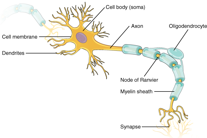
The figure represents a neuron of a human brain. Human brain learns through experience. This learning is done, by adjusting certain events and giving them priority. This process of giving priority to any event is done by giving weights to each of the event, and these weights are then passed to other neurons through a phenomenon called synapse. Similiar to the above concept, ANN works. Consider the figure below:

There are 3 layers,
- Input Layer - takes the input
- Hidden Layer - adjust the weights/ learning phase
- Output Layer - displays the result
ANNs gather their knowledge by detecting the patterns and relationships in data and learn (or are trained) through experience, not from programming. An ANN is formed from hundreds of single units, artificial neurons or processing elements (PE), connected with coefficients (weights), which constitute the neural structure and are organised in layers. The power of neural computations comes from connecting neurons in a network. Each PE has weighted inputs, transfer function and one output. The behavior of a neural network is determined by the transfer functions of its neurons, by the learning rule, and by the architecture itself. The weights are the adjustable parameters and, in that sense, a neural network is a parameterized system. The weighed sum of the inputs constitutes the activation of the neuron. The activation signal is passed through transfer function to produce a single output of the neuron. Transfer function introduces non-linearity to the network. During training, the inter-unit connections are optimized until the error in predictions is minimized and the network reaches the specified level of accuracy. Once the network is trained and tested it can be given new input information to predict the output.
We calculate the total error at the output nodes and propagate these errors back through the network using Backpropagation to calculate the gradients. Then we use an optimization method such as Gradient Descent to ‘adjust’ all weights in the network with an aim of reducing the error at the output layer.

Suppose that the new weights associated with the node in consideration are w4, w5 and w6 (after Backpropagation and adjusting weights). If we now input the same example to the network again, the network should perform better than before since the weights have now been adjusted to minimize the error in prediction. As shown in Figure 7, the errors at the output nodes now reduce to [0.2, -0.2] as compared to [0.6, -0.4] earlier. This means that our network has learnt to correctly classify our first training example.

We repeat this process with all other training examples in our dataset. Then, our network is said to have learnt those examples.

Full connection represent the overall connection for the Convolutional Neural Networks - (CNN + ANN) Consider an example of predicting whether a car is present in an image or not. For this purpose we train our Convolutional layer and reduce its dimenstions by max pooling followed by flattening. Now this reduction of dimensions is done so that, ANN can take that as an input. ANN cannot take an input directly in the form of an image, so first we have to reduce its dimensions. After Flattening of the image, we get a form in which ANN can take the input. At the end we can also apply softmax function, in order to get the output in the form of binary, and hence it reduces the loss.

The full connection can be seen in the above figure.