Data Modeling.md

footer: Riccardo Tommasini - riccardo.tommasini@ut.ee - @rictomm slide-dividers: #, ##, ### slidenumbers: true autoscale: true theme: Plain Jane

Data Engineering: Data Modeling

LTAT.02.007

Ass Prof. Riccardo Tommasini

Assistants: Fabiano Spiga, Mohamed Ragab, Hassan Eldeeb

• https://courses.cs.ut.ee/2020/dataeng
• Forum
• Moodle

What is Data Modeling?

It is the process of defining the structure of the data for the purpose of communicating¹ or to develop an information systems².

What is a data model?

A data model represents the structure and the integrity of the data elements of a (single) applications 2

Data models provide a framework for data to be used within information systems by providing specific definition and format.

The literature of data management is rich of data models that aim at providing increased expressiveness to the modeler and capturing a richer set of semantics.

---

Data models are perhaps the most important part of developing software. They have such a profound effect not only on how the software is written, but also on how we think about the problem that we are solving¹. --Martin Kleppmann

Any Example?

---

Level of Data Modeling

Conceptual: The data model defines WHAT the system contains.

^ Conceptual model is typically created by Business stakeholders and Data Architects. The purpose is to organize, scope and define business concepts and rules. Definitions are most important this level.

Logical: Defines HOW the system should be implemented regardless of the DBMS.

^ Logical model is typically created by Data Architects and Business Analysts. The purpose is to developed technical map of rules and data structures. Business rules, relationships, attribute become visible. Conceptual definitions become metadata.

Physical: This Data Model describes HOW the system will be implemented using a specific DBMS system ³.

^ Physical model is typically created by DBA and developers. The purpose is actual implementation of the database. Trade-offs are explored by in terms of data structures and algorithms.

A Closer Look⁴

^ The variety of data available today encourages the design and development of dedicated data models and query languages that can improve both BI as well as the engineering process itself.

---

---

Conceptual

• Semantic Model (divergent)

  • Describes an enterprise in terms of the language it uses (the jargon).
  • It also tracks inconsistencies, i.e., semantic conflicts

• Architectural Model (convergent)

  • More fundamental, abstract categories across enterprise

Logical

Already bound to a technology, it typically refers already to implementation details

• Relational
• Hierarchical
• Key-Value
• Object-Oriented
• Graph

^ Since it has a physical bias, you might be tempted to confuse this with the physical model, but this is wrong.

Physical

The physical level describes how data are Stored on a device.

• Data formats
• Distribution
• Indexes
• Data Partitions
• Data Replications

...an you are in the Big Data World

A Question

Why should you, an application developer a data engineer, care how the database handles storage and retrieval internally? --Martin Kleppmann

I mean, you’re probably not going to implement your own storage engine from scratch...

---

The Students

---

But...

• You do need to select a storage engine that is appropriate for your application, from the many that are available
• You need to tune a storage engine to perform well on your kind of workload
• You are going to experiment with different access patterns and data formats

Therefore, you must have a rough idea of what the storage engine is doing under the hood

---

Also the Students

Data Formats

• In memory, data are kept in objects, structs, lists, arrays, hash tables, trees, and so on. These data structures are optimized for efficient access and manipulation by the CPU (typically using pointers).
• On Disk (or over the network), data are encoded into a self-contained sequence of bytes (for example, a JSON document).

Encoding and decoding

Encoding is the translation from the in-memory representation to a byte sequence (also known as serialization or marshalling)

Decoding is the reverse translation from the byte sequence to a memory layout (also known as parsing, deserialization, unmarshalling)

The encoding is often tied to a particular programming language, and reading the data in another language is very difficult

Memory vs Disk

Data layout is much less important in memory than on disk.

An efficient disk-resident data structure must allow quick access to it, i.e., find a way to serialize and deserialize data rapidly and in a compacted way.

In general, pointers do not make sense outside memory, thus the sequence-of-bytes representation looks quite different from the data structures that are normally used in memory.

Popular (textual) File Formats

JSON

• has a schema
• cannot distinguish between integers and floating-point numbers
• have good support for Unicode character string
• do not support sequences of bytes without a character encoding XML
• has a schema
• cannot distinguish between a number and a string
• have good support for Unicode character string
• do not support sequences of bytes without a character encoding CSV
• cannot distinguish between a number and a string
• does not have any schema

Avro

Avro is a binary encoding format that uses a schema to specify the structure of the data being encoded.

Avro's encoding consists only of values concatenated together, and the there is nothing to identify fields or their datatypes in the byte sequence.

---

Avro Schema Definition

record Person {     
 string userName;
 union { null, long } favoriteNumber = null;     
 array<string>        interests; 
}

---

Example

Source

---

Encoding and Decoding

• Encoding requires the writer's schema
• Decoding requires the reader’s schema.
• Avro does not require that the writer’s schema and the reader’s schema are the same, they only need to be compatible

---

Schema Evolution Rules

• If the code reading the data encounters a field that appears in the writer’s schema but not in the reader’s schema, it is ignored.
• If the code reading the data expects some field, but the writer’s schema does not contain a field of that name, it is filled in with a default value declared in the reader’s schema.

---

Compatibility

• forward compatibility: there is a new version of the writer's schema and an old version of the reader's schema
• backwards compatibility: there is a new version of the reader's schema and an old version of the writer's schema

Worth Mentioning⁵

• Apache Thrift and Protocol Buffers are binary encoding libraries
  • require a schema for any data that is encoded.
  • come with a code generation tool that takes a schema definitions to reproduce the schema in various programming languages

[.column]

struct Person {   
		1: required string userName,   
		2: optional i64    favoriteNumber,
		3: optional list<string> interests 
}

[.column]

message Person {
	required string user_name       = 1;     
	optional int64  favorite_number = 2;     
	repeated string interests       = 3; 
}

Distribution

CAP Theorem (Brewer’s Theorem)

It is impossible for a distributed computer system to simultaneously provide all three of the following guarantees:

• Consistency: all nodes see the same data at the same time
• Availability: Node failures do not prevent other survivors from continuing to operate (a guarantee that every request receives a response whether it succeeded or failed)
• Partition tolerance: the system continues to operate despite arbitrary partitioning due to network failures (e.g., message loss)

A distributed system can satisfy any two of these guarantees at the same time but not all three.

---

[.text: #ffffff] source

The network is not reliable

In a distributed system, **a network (of networks) ** failures can, and will, occur.

We cannot neglect Partition Tolerance

The remaining option is choosing between Consistency and Availability.

---

We cannot neglect Partition Tolerance

Not necessarily in a mutually exclusive manner:

• CP: A partitioned node returns
  • the correct value
  • a timeout error or an error, otherwise
• AP: A partitioned node returns the most recent version of the data, which could be stale.

Indexing

• Indices are critical for efficient processing of queries in (any kind of) databases.
• basic idea is trading some computational cost for space, i.e., materialize a convenient data structure to answer a set of queries.
• The caveat is that we must maintain indexes up-to-date upon changes

^

• Without indices, query cost will blow up quickly making the database unusable
• databases don’t usually index everything by default

Basics Terms

• Ordered indices. Based on a sorted ordering of the values.

• Hash indices. Using an hash-function that assigns values across a range of buckets.

• Primary Index: denotes an index on a primary key

• Secondary Index: denotes an index on non primary values

Data Replication

Replication means keeping a copy of the same data on multiple machines that are connected via a network

Reasons for Replication

• Increase data locality
• Fault tolerance
• Concurrent processing (read queries)

^

• To keep data geographically close to your users (and thus reduce access latency)
• To allow the system to continue working even if some of its parts have failed (and thus increase availability)
• To scale out the number of machines that can serve read queries (and thus increase read throughput)

Approaches

• Synchronous vs Asynchronous Replication

  • The advantage of synchronous replication is that the follower is guaranteed to have an up-to-date copy
  • The advantage of asynchronous replication is that follower's availability is not a requirement (cf CAP Theorem)

• Leader - Follower (Most common cf Kafka)

Leaders and Followers

• One of the replicas is designated as the leader
• Write requests go to the leader
• leader sends data to followers for replication
• Read request may be directed to leaders or followers

---

Source is ³

Caveats

Only one: handling changes to replicated data is extremely hard.

Data Partitioning (Sharding)

breaking a large database down into smaller ones

^ For very large datasets, or very high query throughput, that is not sufficient

Reasons for Partitioning

• The main reason for wanting to partition data is scalability³

^

• Different partitions can be placed on different nodes in a shared-nothing cluster
• Queries that operate on a single partition can be independently executed. Thus, throughput can be scaled by adding more nodes.

What to know

• If some partitions have more data or queries than others the partitioning is skewed
• A partition with disproportionately high load is called a hot spot
• For reaching maximum scalability (linear) partitions should be balanced

Let's consider some partitioning strategies, for simplicity we consider Key,Value data.

Partitioning Strategies

• Round-robin randomly assigns new keys to the partitions.
  • Ensures an even distribution of tuples across nodes;
• Range partitioning assigns a contiguous key range to each node.
  • Not necessarily balanced, because data may not be evenly distributed
• Hash partitioning uses a hash function to determine the target partition. - If the hash function returns i, then the tuple is placed

Let's take a step back

[.header: #ffffff] [.text: #ffffff]

---

To the future

[.header: #ffffff] [.text: #ffffff]

^ Joke Explained: because we will discuss Processing later

Let's Talk about Workloads

^

• OLTP systems are usually expected to be highly available and to process transactions with low latency, since they are often critical to the operation of the business.
• OLAP queries are often written by business analysts, and feed into reports that help the management of a company make better decisions (business intelligence).

Online Transactional Processing

Because these applications are interactive, the access pattern became known as online

Transactional means allowing clients to make low-latency reads and writes—as opposed to batch processing jobs, which only run periodically (for example, once per day).

Refresh on ACID Properties

• ACID, which stands for Atomicity, Consistency, Isolation, and Durability⁶

• Atomicity refers to something that cannot be broken down into smaller parts.

  • It is not about concurrency (which comes with the I)

• Consistency (overused term), that here relates to the data invariants (integrity would be a better term IMHO)

• Isolation means that concurrently executing transactions are isolated from each other.

  • Typically associated with serializability, but there weaker options.

• Durability means (fault-tolerant) persistency of the data, once the transaction is completed.

^ The terms was coined in 1983 by Theo Härder and Andreas Reuter ⁶

Online Analytical Processing

An OLAP system allows a data analyst to look at different cross-tabs on the same data by interactively selecting the attributes in the cross-tab

Statistical analysis often requires grouping on multiple attributes.

Example⁷

Consider this is a simplified version of the sales fact table joined with the dimension tables, and many attributes removed (and some renamed)

sales (item_name, color, clothes_size, quantity)

---

item_name	color	clothes_size	quantity
dress	dark	small	2
dress	dark	medium	6
...	...	...	...
pants	pastel	medium	0
pants	pastel	large	1
pants	white	small	3
pants	white	medium	0
shirt	white	medium	1
...	...	...	...
shirt	white	large	10
skirt	dark	small	2
skirt	dark	medium	5
...	...	...	...

Cross-tabulation of sales by item name and color

	dark	pastel	white	total
skirt	8	35	10	53
dress	20	11	5	36
shirt	22	4	46	72
pants	23	42	25	90
total	73	92	102	267

columns header: color rows header: item name

Data Cube⁷

• It is the generalization of a Cross-tabulation

Cheat Sheet of OLAP Operations⁷

• Pivoting: changing the dimensions used in a cross-tab
  • E.g. moving colors to column names
• Slicing: creating a cross-tab for fixed values only
  • E.g fixing color to white and size to small
  • Sometimes called dicing, particularly when values for multiple dimensions are fixed.
• Rollup: moving from finer-granularity data to a coarser granularity
  • E.g. aggregating away an attribute
  • E.g. moving from aggregates by day to aggregates by month or year
• Drill down: The opposite operation - that of moving from coarser granularity data to finer-granularity data

Summary OLTP vs OLAP³

Property	OLTP	OLAP
Main read pattern	Small number of records per query, fetched by key	Aggregate over large number of records
Main write pattern	Random-access, low-latency writes from user input	Bulk import (ETL) or event stream
Primarily used by	End user/customer, via web application	Internal analyst, for decision support
What data represents	Latest state of data (current point in time)	History of events that happened over time
Dataset size	Gigabytes to terabytes	Terabytes to petabytes

---

Modeling for (relational) Database⁸

• Works in phases related to the aforementioned levels of abstractions
• Uses different data models depending on the need:
  • Relational, Graph, Document...
• Tries to avoid two major pitfalls:
  • Redundancy: A design should not repeat information
  • Incompleteness: A design should not make certain aspects of the enterprise difficult or impossible to model
• Optimized for OLTP

^ The biggest problem with redundancy is that information may become inconsistent in case of update

---

Before, let's refresh

---

Relational Database

A relational database consists of…

• a set of relations (tables)
• a set of integrity constraints

If the database satisfies all the constraints we said it is in a valid state.

An important distinction regards the database schema, which is the logical design of the database, and the database instance, which is a snapshot of the data in the database at a given instant in time.

Relational Model ⁹

A formal mathematical basis for databases based on set theory and first-order predicate logic

Underpins of SQL

Relation

Relation R is a set of tuples (d₁, d₂, ..., d_n), where each element d_j is a member of D_j, a data domain.

A Data Domain refers to all the values which a data element may contain, e.g., N.

Note that in the relational model the term relation is used to refer to a table, while the term tuple is used to refer to a row

^ In mathematical terms, a tuple indicates a sequence of values. A relationship between n values is represented mathematically by an n-tuple of values, that is, a tuple with n values, which corresponds to a row in a table.

---

---

Relation Schema

• corresponds to the notion of type in programming languages
• consists of a list of attributes and their corresponding domains
• a relation instance corresponds to the programming-language no- tion of a value of a variable

---

Keys

• A superkey is a set of one or more attributes that, taken collectively, allow us to identify uniquely a tuple in the relation
• candidate keys are superkeys for which no proper subset is a superkey
• primary key is the chosen candidate key
• foreign key is s set of attributes from a referenced relation.

^ If K is a superkey, then so is any superset of K

---

---

Relational Algebra (On Practice)

is a procedural language consisting of a six basic operations that take one or two relations as input and produce a new relation as their result:

• select: σ
• project: ∏
• union: ∪
• set difference: –
• Cartesian product: x
• rename: ρ

^ Question: What is an algebra?

---

Two Sets

---

Intersection

---

Difference

---

Union

---

---

Projection

---

Selection

---

Natural JOIN

---

Entity-Relationship (ER) Model

• Outputs a conceptual schema.
• The ER data model employs three basic concepts:
  • entity sets
  • relationship sets and
  • attributes.
• It is also associated with diagrammatic representation try out

Entities And Entity Sets

An entity can be any object in the real world that is distinguishable from all other objects.

An entity set contains entities of the same type that share the same properties, or attributes.

NB We work at set level

^ Ask the students Examples of entities: - University - Department - Persons - Courses

• Examples of entity sets
  • Professors and Students
  • Data Science courses: curriculums

---

Syntax

^ fields are what we call attributes

Relationships and Relationship Sets

A relationship is an association among several entities.

A relationship set is a set of relationships of the same type.

^ Examples of entities: - advisor - attendee - enrollment

Intuition

---

Syntax


^^ ER works under the assumption that most relationship sets in a database system are binary. Relationships between more than two entity sets are rare.

Attributes and Values

attributes. Attributes are descriptive properties possessed by each member of an entity set.

Each entity has a value for each of its attributes.

Also relationships may have attributes called descriptive attributes.

Intuition

---

Syntax

Cardinality

For a binary relationship set the mapping cardinality must be one of the following types:

• One to one
• One to many
• Many to one
• Many to many

---

Cardinality Visualized

• (a) One to One
• (b) One to Many

---

Cardinality Visualized

• (a) Many to One
• (b) Many to Many

University of Tartu Example

source

---

One to Many


A (full) professor has one office an office hosts one full professor

---

One to Many

A Dean is associated with many institutes An Institute has only one dean

---

Many to One

A professor advises many students but a student has only one advisor.

^ Many students share the same advisor but they only have one.

---

Many to Many

A course is associated to many institute in the context of a curriculum An institute offers many courses within a curriculum

Keys

• Provide a way to specify how entities and relations are distinguished.
• Primary key for Entity Sets
  • By definition, individual entities are distinct (set)
  • From database perspective, the differences among them must be expressed in terms of their attributes
• Primary Key for Relationship Sets
  • We use the individual primary keys of the entities in the relationship set.
  • The choice depends on the mapping cardinality of the relationship set.

---

Choice of Primary key for Binary Relationship

• One-to-one relationships. The primary key of either one of the participating entity sets forms a minimal superkey, and either one can be chosen as the primary key.
• One-to-Many relationships and Many-to-one relationships
  • The primary key of the “Many” side is a minimal superkey and is used as the primary key.
• Many-to-Many relationships:
  • The preceding union of the primary keys is a minimal superkey and is chosen as the primary key.

---

Weak Entity Sets

• A weak entity set is one whose existence is dependent on another entity, called its identifying entity

• A weak entity set is one whose existence is dependent on another entity, called its identifying entity

Summary of Symbols

---

From ER to Relational Model

• Entity and relationship sets can be expressed as relation schemas that represent the contents of the database.

• A database which conforms to an E-R diagram can be represented by a collection of schemas.

---

Reduction of Entities

• For each entity set there is a unique schema with the same name

• Each schema has a number of columns (generally corresponding to attributes), which have unique names

Professor(ID,Name,Age) Student(ID,Name,GPA)

^ Weak entities set becomes a relation that includes a column for the primary key of the identifying entity.

---

Reduction of Relationships

[.column]

• For each relationship set there is a unique schema with the same name

• A many-to-many relationship (figure) is represented as a schema with attributes for the primary keys of the two participating entity sets, and any descriptive attributes of the relationship set.

[.column]

Curriculum(Institute_ID,Course_ID)

---

Reduction of Relationships

• Many-to-one and one-to-many** relationship can be represented by adding an extra attribute to the "many" side

• For one-to-one relationship, either side can be chosen to act as the "many" side

Normalisation

• Typically decomposes tables to avoid redundancy
• Spans both logical and physical database design
• Aims at improving the database design

---

Goals

• Make the schema informative
• Minimize information duplication
• Avoid modification anomalies
• Disallow spurious tuples

---


---


---

---

Normal Forms (Refresh)

• First Normal Form (1NF)
  • A table has only atomic valued columns.
  • Values stored in a column should be of the same domain
  • All the columns in a table should have unique names.
  • And the order in which data is stored, does not matter.
• Second Normal Form (2NF)
  • A table is in the First Normal form and every non-prime attribute is fully functional dependent¹⁰ on the primary key
• Third Normal Form (3NF)
  • A table is in the Second Normal form and every non-prime attribute is non-transitively dependent¹¹ on every key

---

Modeling for Database: A note on Storage

• Storage is laid out in a row-oriented fashion
• For relational this is as close as the tabular representation
• All the values from one row of a table are stored next to each other.
• This is true also for some NoSQL (we will see it again)
  • Document databases stores documents a contiguous bit sequence

Data Modeling for Data Warehouse

• Works in phases related to the aforementioned levels of abstractions
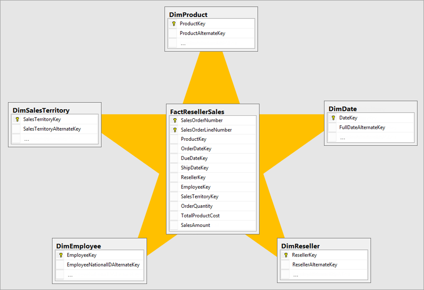
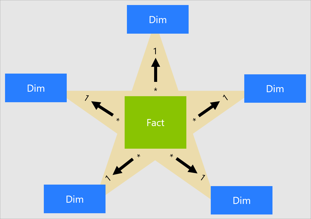
• Less diversity in the data model, usually relational in the form of a star schema (also known as dimensional modeling¹²).
• Redundancy and incompleteness are not avoided, fact tables often have over 100 columns, sometimes several hundreds.
• Optimized for OLAP

^

• The data model of a data warehouse is most commonly relational, because SQL is generally a good fit for analytic queries.
• Do not associate SQL with analytic, it depends on the data modeling.

A Star is Born

[.column]

[.column]

A Star is Born

[.column]

[.column]

Dimensional Modelling

Four-Step Dimensional Design Process

1. Select the business process.
2. Declare the grain.
3. Identify the dimensions.
4. Identify the facts.

Mandatory Read

^

• Business processes are critical activities that your organization performs, e.g., registering students for a class.
• The grain establishes exactly what a single fact table row represents. Three common grains categorize all fact tables: transactional, periodic snapshot, or accumulating snapshot.
• Dimensions provide context to business process events, e.g., who, what, where, when, why, and how.
• :wq
• Facts are the measurements that result from a business process event and are almost always numeric.

Dimensional Modelling: Fact Table

A fact table contains the numeric measures produced by an operational measurement event in the real world.

A single fact table row has a one-to-one relationship to a measurement event as described by the fact table’s grain.

A surrogate key is a unique identifier that you add to a table to support star schema modeling. By definition, it's not defined or stored in the source data

Dimensional Modelling: Dimension Table

Dimension tables contain the descriptive attributes used by BI applications for filtering and grouping the facts.

Every dimension table has a single primary key column , which is embedded as a foreign key in any associated fact table.

The 10 Essential Rules of Dimensional Modeling (Read)¹³

1. Load detailed atomic data into dimensional structures.
2. Structure dimensional models around business processes.
3. Ensure that every fact table has an associated date dimension table.
4. Ensure that all facts in a single fact table are at the same grain or level of detail.
5. Resolve many-to-many relationships in fact tables.
6. Resolve many-to-one relationships in dimension tables.
7. Store report labels and filter domain values in dimension tables.
8. Make certain that dimension tables use a surrogate key.
9. Create conformed dimensions to integrate data across the enterprise.
10. Continuously balance requirements and realities to deliver a DW/BI solution that’s accepted by business users and that supports their decision-making.

The Traditional RDBMS Wisdom Is (Almost Certainly) All Wrong¹⁴

A note on Storage

• Data warehouse typically interact with OLTP database to expose one or more OLAP system.
• Such OLAP system adopt storage optimized for analytics, i.e., Column Oriented
• The column-oriented storage layout relies on each column file containing the rows in the same order.
• Not just relational data, e.g., Apache Parquet

Data Modeling for Big Data

^ The Data Landscape: Variety is the Driver

The Data Landscape

^ Structured data are organized and labeled according to a precise model (e.g., relational data) ^ Unstructured data, on the other hand, are not constrained (e.g., text, video, audio) ^ In between, there are many form of semi-structured data, e.g., JSON and XML, whose models do not impose a strict structure but provide means for validation.

Big Data Storage

• Distributed File Systems, e.g., HDFS
• Distributed Databases, e.g., VoltDB
• Key-Value Storage Systems, e.g., Redis or Cassandra
• Queues, e.g., Pulsar or Kafka

^ A distributed file system stores files across a large collection of machines while giving a single-file-system view to clients.

Let's Talk Distributed File Systems

A distributed file system stores files across a large collection of machines while giving a single-file-system view to clients.

Hadoop Distributed File System (HDFS)¹⁵

• Abstracts physical location (Which node in the cluster) from the application
• Partition at ingestion time
• Replicate for high-availability and fault tolerance

Design Objectives

• Partition and distribute a single file across different machines
• Favor larger partition sizes
• Data replication
• Local processing (as much as possible)

Optimizations

• Reading sequentially versus (random access and writing)
• No updates on files
• No local caching

HDFS Architecture¹⁶

HDFS Files

• A single large file is partitioned into several blocks
  • Size of either 64 MB or 128MB
  • Compare that to block sizes on ordinary file systems
  • This is why sequential access is much better as the disk will make less numbers of seeks

^ Question: What would be the costs/benefits if we use smaller block sizes?

Data Node

• It stores the received blocks in a local file system;
• It forwards that portion of data to the next DataNode in the list.
• The operation is repeated by the next receiving DataNode until the last node in the replica set receives data.

Name Node

• A single node that keeps the metadata of HDFS
  • Keeps the metadata in memory for fast access
  • Periodically flushes to the disk (FsImage file) for durability
  • Name node maintains a daemon process to handle the requests and to receive heartbeats from other data nodes

^ - In some high-availability setting, there is a secondary name node - As a name node can be accessed concurrently, a logging mechanism similar to databases is used to track the updates on the catalog.

HDFS Federation

• By default, HDFS has a single NameNode. What is wrong with that? If NameNode daemon process goes down, the cluster is inaccessible

• A solution: HDFS Federation

  • Namespace Scalability: Horizontal scalability to access meta data as to access the data itself
  • Performance: Higher throughput as NameNodes can be queried concurrently
  • Isolation: Serve blocking applications by different NameNodes

• Is it more reliable?

Writing to HDSF

• When a client is writing data to an HDFS file, this data is first written to a local file.
• When the local file accumulates a full block of data, the client consults the NameNode to get a list of DataNodes that are assigned to host replicas of that block.
• The client then writes the data block from its local storage to the first DataNode in 4K portions.

Writing a File to HDSF Cont.

• This DataNode stores data locally without sending it any further
• If one of the DataNodes fails while the block is being written, it is removed from the pipeline
• The NameNode re-replicates it to make up for the missing replica caused by the failed DataNode
• When a file is closed, the remaining data in the temporary local file is pipelined to the DataNodes
• If the NameNode dies before the file is closed, the file is lost.

Replica Placement

• Replica placement is crucial for reliability of HDFS
  • Should not place the replicas on the same rack
• All decisions about placement of partitions/replicas are made by the NameNode
• NameNode tracks the availability of Data Nodes by means of Heartbeats
  • Every 3 seconds, NameNode should receive a heartbeat and a block report from each data node
  • Block report allows verifying the list of stored blocks on the data node
  • Data node with a missing heartbeat is declared dead, based on the catalog, replicas missing on this node are made up for through NameNode sending replicas to other available data nodes

HDFS High-availability

• Each NameNode is backed up with a slave other NameNode that keeps a copy of the catalog

• The slave node provides a failover replacement of the primary NameNode

• Both nodes must have access to a shared storage area

• Data nodes have to send heartbeats and block reports to both the master and slave NameNodes.

Data Modeling Techniques

According to Len Silverston (1997) only two modeling methodologies stand out, top-down and bottom-up[^14].

Data Modeling Techniques¹⁷

• Entity-Relationship (ER) Modeling¹⁸ prescribes to design model encompassing the whole company and describe enterprise business through Entities and the relationships between them - it complies with 3rd normal form - tailored for OLTP

• Dimensional Modeling (DM)¹⁹ focuses on enabling complete requirement analysis while maintaining high performance when handling large and complex (analytical) queries

  • The star model and the snowflake model are examples of DM
  • tailored for OLAP

• Data Vault (DV) Modeling⁹ focuses on data integration trying to take the best of ER 3NF and DM - emphasizes establishment of an auditable basic data layer focusing on data history, traceability, and atomicity - one cannot use it directly for data analysis and decision making

Event Sourcing²⁰

The fundamental idea of Event Sourcing is ensuring that every change to the state of an application is captured in an event object,

Event objects are immutable and stored in the sequence they were applied for the same lifetime as the application state itself.

Events

Events are both a fact and a notification.

They represent something that happened in the real world but include no expectation of any future action.

They travel in only one direction and expect no response (sometimes called “fire and forget”), but one may be “synthesized” from a subsequent event.

---

---

---

---

History of Data Models²¹

---

The World's most simple database

#!/bin/bash 

db_set () {     
	echo "$1,$2" >> db 

} 

db_get () { 
	grep "^$1," db | sed -e "s/^$1,//" | tail -n 1 
}

^ db_set is appending data to a file. This is generally quite efficient. Indeed, many databases internally use the same strategy, but it is not a normal file, is a log.

The Log

A log is an append-only sequence of records. It doesn’t have to be human-readable; it might be binary and intended only for other programs to read.

^ Questions:

• What is the cost of lookup O(n)
• What is the cost of write O(1)
• What is the cost of read from the head O(1).

Footnotes

1. between functional and technical people to show data needed for business processes ↩ ↩²

2. between components of the information system, how data is stored and accessed. ↩

3. Designing Data-Intensive Applications ↩ ↩² ↩³ ↩⁴

4. physical ↩

5. Chapter 4. Encoding and Evolution ↩

6. Theo Härder and Andreas Reuter: “Principles of Transaction-Oriented Database Recovery,” ACM Computing Surveys, volume 15, number 4, pages 287–317, December 1983. doi:10.1145/289.291 ↩ ↩²

7. Database System Concepts Seventh Edition Avi Silberschatz Henry F. Korth, S. Sudarshan McGraw-Hill ISBN 9780078022159 link ↩ ↩² ↩³

8. Also known as Database Design ↩

9. Extra Read Codd, Edgar F. "A relational model of data for large shared data banks." Communications of the ACM 13.6 (1970): 377-38z ↩ ↩²

10. $$X \rightarrow Y, \forall A \in X ((X -{A}) \nrightarrow Y)$$ ↩

11. ↩

12. Ralph Kimball and Margy Ross: The Data Warehouse Toolkit: The Definitive Guide to Dimensional Modeling, 3rd edition. John Wiley & Sons, July 2013. ISBN: 978-1-118-53080-1 ↩

13. https://www.kimballgroup.com/2009/05/the-10-essential-rules-of-dimensional-modeling/ ↩

14. Source with slides: The Traditional RDBMS Wisdom Is (Almost Certainly) All Wrong,” presentation at EPFL, May 2013 ↩

15. Inspired by Google File System ↩

16. Figure 2-1 in book Professional Hadoop Solutions ↩

17. source ↩

18. by Bill Inmon ↩

19. Ralph Kimball, book ‘The Data Warehouse Toolkit — The Complete Guide to Dimensional Modeling" ↩

20. Martin Fowler, link ↩

21. slides & video by Donna Burbank ↩